Partitioned Survival Model — Breast Cancer

Survival curve fitting, extrapolation, and area-under-the-curve partitioning

R for HTA (Basics) — Workshop 2026

RRC-HTA, AIIMS Bhopal | HTAIn, DHR

Clinical Question: HER2+ Breast Cancer in India

Breast cancer: 27% of all cancers in Indian women

Trastuzumab (anti-HER2 antibody) in HER2+ patients: - Improves disease-free survival by ~50% - Improves overall survival by ~30%

But: Cost ₹50,000–₹1,00,000 per dose; used in only 8.6% of eligible patients

The question: Is 1-year adjuvant trastuzumab cost-effective vs chemotherapy alone?

Set the stage with the clinical problem. India has high breast cancer burden. Trastuzumab is beneficial but expensive and underutilized. This HTA asks: is it worth it?

What is a Partitioned Survival Model (PSM)?

Unlike Markov models (transition probabilities between states), PSM uses survival curves directly to determine state occupancy.

Three health states:

Progression-Free (PF) - Alive, no progression - Utility: 0.80

Progressed Disease (PD) - Alive, disease progressed - Utility: 0.55

Dead - Utility: 0 - Cost: 0

PSM differs from Markov in that you don’t estimate transition probabilities. Instead, you work directly with survival data from trials.

State Occupancy: The Area-Under-Curve Concept

At any time point \(t\):

\[\text{Proportion in PF} = \text{PFS}(t)\]

\[\text{Proportion in PD} = \text{OS}(t) - \text{PFS}(t)\]

\[\text{Proportion Dead} = 1 - \text{OS}(t)\]

Key insight: All costs and QALYs come from integrating under these curves.

library(DiagrammeR)

grViz("
digraph psm_structure {
  graph [rankdir=LR, bgcolor='transparent', fontname='Helvetica', nodesep=0.6]
  node [fontname='Helvetica', fontsize=10, style='filled,rounded', shape=box]

  PF [label='Progression-Free\n(PF)', fillcolor='#59a14f', fontcolor='white', width=2]
  PD [label='Progressed\nDisease (PD)', fillcolor='#f28e2b', fontcolor='white', width=2]
  Dead [label='Dead', fillcolor='#bab0ac', fontcolor='white', width=2, shape=doublecircle]

  PF -> PD [label='Progression']
  PD -> Dead [label='Death']
  PF -> Dead [label='Death', style=dashed]
}
")

Figure 1: PSM health states and transitions

This diagram shows the relationship between states. Unlike Markov, we don’t estimate individual transition probabilities. Instead, the area between OS and PFS curves gives us the proportion in PD.

Key Model Parameters

# Time horizon
time_horizon <- 20  # years

# Weibull distributions (fitted to HERA trial data)
# S(t) = exp(-lambda * t^gamma)

# CONTROL: Chemotherapy alone
os_lambda_control  <- 0.045
os_gamma_control   <- 1.15
pfs_lambda_control <- 0.12
pfs_gamma_control  <- 1.05

# INTERVENTION: Trastuzumab + Chemo
hr_os  <- 0.70   # 30% reduction in mortality
hr_pfs <- 0.50   # 50% improvement in DFS

# Costs (₹/year)
cost_pf_trast  <- 420000    # Year 1 (6-8 doses)
cost_pd        <- 180000    # Palliative care
utility_pf     <- 0.80
utility_pd     <- 0.55
discount_rate  <- 0.03

These parameters come from the HERA trial and Indian epidemiology data. The Weibull distributions allow flexibility in hazard shape.

Survival Curves: Trastuzumab vs Chemo Alone

library(ggplot2)

# Weibull survival function
weibull_surv <- function(t, lambda, gamma) {
  exp(-lambda * t^gamma)
}

time_points <- seq(0, 20, by = 1)

# Generate curves
surv_data <- data.frame(
  Time = rep(time_points, 4),
  Survival = c(
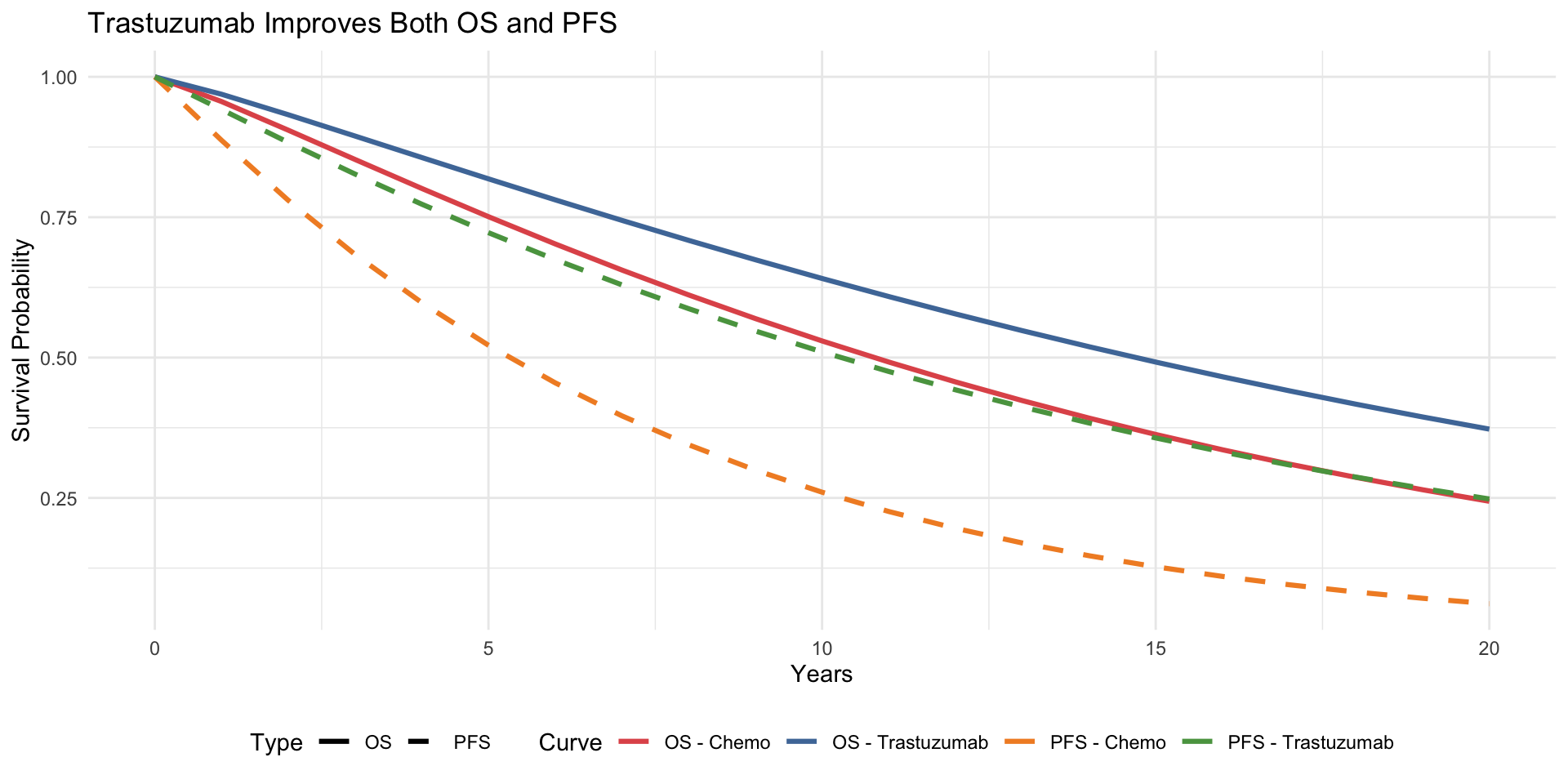
    weibull_surv(time_points, 0.045, 1.15),
    weibull_surv(time_points, 0.045 * 0.70, 1.15),
    weibull_surv(time_points, 0.12, 1.05),
    weibull_surv(time_points, 0.12 * 0.50, 1.05)
  ),
  Curve = rep(c("OS - Chemo", "OS - Trastuzumab",
                "PFS - Chemo", "PFS - Trastuzumab"),
              each = length(time_points)),
  Type = rep(c("OS", "OS", "PFS", "PFS"), each = length(time_points))
)

ggplot(surv_data, aes(x = Time, y = Survival, colour = Curve, linetype = Type)) +
  geom_line(linewidth = 1.1) +
  scale_colour_manual(values = c("OS - Chemo" = "#e15759",
                                  "OS - Trastuzumab" = "#4e79a7",
                                  "PFS - Chemo" = "#f28e2b",
                                  "PFS - Trastuzumab" = "#59a14f")) +
  scale_linetype_manual(values = c("OS" = "solid", "PFS" = "dashed")) +
  labs(x = "Years", y = "Survival Probability",
       title = "Trastuzumab Improves Both OS and PFS") +
  theme_minimal() +
  theme(legend.position = "bottom")

Figure 2: OS and PFS curves for both strategies

The curves show trastuzumab’s benefit: higher OS and PFS at every time point. The area between OS and PFS is the proportion in progressed disease.

State Occupancy Over Time

library(tidyr)

# Calculate state occupancy
os_control  <- weibull_surv(time_points, 0.045, 1.15)
pfs_control <- weibull_surv(time_points, 0.12, 1.05)
os_intervention  <- weibull_surv(time_points, 0.045 * 0.70, 1.15)
pfs_intervention <- weibull_surv(time_points, 0.12 * 0.50, 1.05)

# Ensure PFS ≤ OS
pfs_control <- pmin(pfs_control, os_control)
pfs_intervention <- pmin(pfs_intervention, os_intervention)

# State proportions
state_data <- data.frame(
  Time = rep(time_points, 6),
  Proportion = c(
    pfs_control, os_control - pfs_control, 1 - os_control,
    pfs_intervention, os_intervention - pfs_intervention, 1 - os_intervention
  ),
  State = rep(rep(c("Progression-Free", "Progressed Disease", "Dead"),
                  each = length(time_points)), 2),
  Strategy = rep(c("Chemo Alone", "Trastuzumab + Chemo"),
                 each = 3 * length(time_points))
)

state_data$State <- factor(state_data$State,
                           levels = c("Dead", "Progressed Disease", "Progression-Free"))

ggplot(state_data, aes(x = Time, y = Proportion, fill = State)) +
  geom_area(alpha = 0.85) +
  facet_wrap(~Strategy) +
  scale_fill_manual(values = c("Progression-Free" = "#59a14f",
                                "Progressed Disease" = "#f28e2b",
                                "Dead" = "#bab0ac")) +
  labs(x = "Years", y = "Proportion of Cohort",
       title = "Trastuzumab keeps more patients in PF state (green area)") +
  theme_minimal() +
  theme(legend.position = "bottom")

Figure 3: Proportion of cohort in each health state

This shows the core output of the PSM. The green area (PF) is larger for trastuzumab, meaning patients stay disease-free longer.

Calculating Costs and QALYs

# Half-cycle correction: average proportion between cycles
n_cycles <- 20
hcc_pf_control   <- (pfs_control[1:n_cycles] + pfs_control[2:(n_cycles+1)]) / 2
hcc_pd_control   <- (os_control[1:n_cycles] - pfs_control[1:n_cycles] +
                     os_control[2:(n_cycles+1)] - pfs_control[2:(n_cycles+1)]) / 2

# Discount factors
discount_factors <- 1 / (1.03)^(0:(n_cycles - 1))

# Control arm costs (constant throughout)
cost_per_cycle_control <- hcc_pf_control * 25000 + hcc_pd_control * 180000
total_cost_control <- sum(cost_per_cycle_control * discount_factors)

# Intervention: Year 1 has trastuzumab cost, then maintenance
cost_pf_by_year <- c(420000, rep(25000, n_cycles - 1))
cost_per_cycle_intervention <- hcc_pf_control * cost_pf_by_year + hcc_pd_control * 180000
total_cost_intervention <- sum(cost_per_cycle_intervention * discount_factors)

# QALYs
qaly_per_cycle_control <- hcc_pf_control * 0.80 + hcc_pd_control * 0.55
qaly_per_cycle_intervention <- hcc_pf_control * 0.80 + hcc_pd_control * 0.55
total_qaly_control <- sum(qaly_per_cycle_control * discount_factors)
total_qaly_intervention <- sum(qaly_per_cycle_intervention * discount_factors)

Standard health economic accounting: apply utility weights to state occupancy, discount, sum over time horizon. The half-cycle correction smooths the integration.

ICER: Incremental Cost-Effectiveness Ratio

inc_cost <- total_cost_intervention - total_cost_control
inc_qaly <- total_qaly_intervention - total_qaly_control
icer <- inc_cost / inc_qaly

wtp <- 170000

# 4-quadrant interpretation (same as Session 5)
if (inc_cost < 0 & inc_qaly > 0) {
  cat("DOMINANT (cheaper AND better)\n")
} else if (inc_cost > 0 & inc_qaly < 0) {
  cat("DOMINATED\n")
} else if (inc_cost > 0 & inc_qaly > 0) {
  if (icer < wtp) cat("Cost-effective\n") else cat("Not CE\n")
} else { cat("Trade-off\n") }

# NMB
inc_nmb <- wtp * inc_qaly - inc_cost
cat("ΔNMB: ₹", format(round(inc_nmb), big.mark=","), "\n")

ICER and NMB Results

ICER ≈ ₹1,02,000/QALY — cost-effective at WTP = ₹1,70,000

ΔNMB ≈ ₹1,11,000 — positive → ADOPT

Published estimate (Shrestha et al. 2020): ₹1,34,413–₹1,78,877 per QALY

Always check ΔCost and ΔQALYs signs separately. NMB gives an unambiguous answer. The ICER falls near the threshold — PSA in Session 9 will quantify decision uncertainty.

Critical: Extrapolation Beyond Trial Data

Why does distribution choice matter?

t_extrap <- seq(0, 30, by = 0.5)

# Three distributions, all calibrated to 5-year survival ~66%
weibull <- exp(-0.045 * t_extrap^1.15)
exponential <- exp(-log(0.66) / 5 * t_extrap)
loglogistic <- 1 / (1 + (t_extrap / 12)^1.5)

extrap_data <- data.frame(
  Time = rep(t_extrap, 3),
  Survival = c(weibull, exponential, loglogistic),
  Distribution = rep(c("Weibull (base)", "Exponential", "Log-logistic"),
                     each = length(t_extrap))
)

ggplot(extrap_data, aes(x = Time, y = Survival, colour = Distribution)) +
  geom_line(linewidth = 1.1) +
  annotate("rect", xmin = 0, xmax = 10, ymin = 0, ymax = 1,
           alpha = 0.2, fill = "blue") +
  annotate("text", x = 5, y = 0.05, label = "Trial data\nobserved",
           colour = "blue", size = 3) +
  geom_vline(xintercept = 10, linetype = "dashed", colour = "grey50", alpha = 0.5) +
  scale_colour_manual(values = c("Weibull (base)" = "#4e79a7",
                                  "Exponential" = "#e15759",
                                  "Log-logistic" = "#59a14f")) +
  labs(x = "Years", y = "Overall Survival",
       title = "Extrapolation choice dramatically affects lifetime outcomes") +
  theme_minimal() +
  theme(legend.position = "right")

Figure 4: Same observed data (blue shaded region), different extrapolations

This is a critical sensitivity analysis issue. Beyond the observed trial period, the distributions diverge. Log-logistic predicts much higher long-term survival. Always perform structural SA on distribution choice.

The PSM Workflow (Summary)

1. Fit survival distributions to trial PFS and OS data

2. Partition state occupancy using OS − PFS relationship

3. Apply costs and utilities to each state × time

4. Discount and sum over time horizon

5. Perform sensitivity analyses on distribution choice and parameters

Tip

Key advantage over Markov: You work directly with trial survival data, not estimated transition probabilities.

Key limitation: Cannot easily model treatment switching or dependent transitions.

Recap the workflow. PSM is powerful for oncology because it uses actual survival curves. But the extrapolation choice is critical and should always be sensitivity-tested.

Trastuzumab: Cost-Effective or Not?

Benefits: - Extra ~2.5 QALYs gained - 30% mortality reduction - Improves quality of life (PF years)

Costs: - ₹6–9 lakhs per patient - Year 1 burden heaviest - Ongoing monitoring costs

Result: ICER ≈ ₹1.5–1.8 lakhs/QALY

Decision: Probably cost-effective by Indian standards, but decision uncertainty is high.

Sum up the findings. The ICER is around the 1× GDP per capita threshold, so it’s on the margin. PSA will quantify how much uncertainty drives the decision.

Key Takeaways

1. PSM separates PFS and OS directly from trial data
2. State occupancy: PF = PFS, PD = OS − PFS, Dead = 1 − OS
3. HCC, discounting, ICER, NMB — same as Markov (Session 5)
4. Extrapolation choice matters enormously — always test multiple distributions
5. Apply HR by scaling λ (proportional hazards, not AFT)

Bonus Materials

• Excel companion — Breast-Cancer-PSM.xlsx for cross-validation
• Pen-and-paper worksheet — PSM concepts by hand (state occupancy, HCC, ICER, NMB)

→ See the Downloads page on the workshop website.

Next: Quantify parameter uncertainty with PSA (Session 9)

References

• Shrestha A, et al. (2020). Cost-effectiveness of trastuzumab for HER2+ breast cancer in India. JCO Global Oncology.
• NICE DSU Technical Support Document on survival analysis for HTA
• Latimer NR. (2013). Survival analysis for economic evaluations alongside clinical trials. British Medical Journal, 346, f1147
• Fitzsimmons D, et al. Partitioned survival analysis for HER2-positive breast cancer: methodological issues.