PSA for the Partitioned Survival Model

Quantifying uncertainty in the trastuzumab cost-effectiveness analysis

R for HTA (Basics) — Workshop 2026

RRC-HTA, AIIMS Bhopal | HTAIn, DHR

Why PSA for the PSM?

Same principle as Session 6 (Markov PSA):

• Define distributions for uncertain parameters
• Sample from those distributions
• Run the model with each sample
• Collect results to build distributions of ICER, costs, QALYs
• Use these to quantify decision uncertainty

Note

PSA methodology is independent of model structure. The workflow is identical for decision trees, Markov models, PSMs, and discrete event simulations.

Reinforce that PSA is universal. We learned it for Markov in Session 6; now we apply it to PSM. The principle never changes.

Parameter Distributions for the Breast Cancer PSM

# HAZARD RATIOS (log-normal distribution)
hr_os_mean   <- log(0.70)    # Log mean
hr_os_sd     <- 0.15         # Log SD
hr_pfs_mean  <- log(0.50)
hr_pfs_sd    <- 0.20

# COSTS (gamma distribution)
cost_pf_trast_yr1_mean <- 420000
cost_pf_trast_yr1_sd   <- 80000   # ~19% of mean

cost_pd_mean <- 180000
cost_pd_sd   <- 40000     # ~22% of mean

# UTILITIES (beta distribution)
utility_pf_mean <- 0.80
utility_pf_sd   <- 0.05

utility_pd_mean <- 0.55
utility_pd_sd   <- 0.08

Which parameter likely causes the most ICER uncertainty?

Answer: Survival parameters (HR, lambda, gamma) — small changes in hazard ratio have large lifetime effects

Set the stage for the parameter distributions. Note that survival parameters (HRs) typically drive more uncertainty than costs or utilities because they affect lifetime accumulation.

Sampling from Distributions: Hazard Ratios

Log-normal distribution for hazard ratios:

# HR ~ log-normal(mu, sigma)
# Sample in log-space, then exponentiate

set.seed(42)

# OS HR
hr_os_sampled <- exp(rnorm(1, mean = log(0.70), sd = 0.15))
cat("Sampled HR_OS:", round(hr_os_sampled, 3), "\n")

# PFS HR
hr_pfs_sampled <- exp(rnorm(1, mean = log(0.50), sd = 0.20))
cat("Sampled HR_PFS:", round(hr_pfs_sampled, 3), "\n")

# Run this many times to see the distribution
n_samples <- 5000
hr_samples <- exp(rnorm(n_samples, mean = log(0.70), sd = 0.15))
cat("\nMedian HR_OS across 5000 samples:", round(median(hr_samples), 3), "\n")
cat("95% CrI: [", round(quantile(hr_samples, 0.025), 3), ", ",
    round(quantile(hr_samples, 0.975), 3), "]\n")

Log-normal is ideal for HR distributions because it keeps values positive and has a flexible right tail. Show how to sample and verify the distribution matches our specified mean/SD.

Sampling from Distributions: Costs (Gamma)

Gamma distribution for costs:

# Convert mean and SD to gamma shape and rate parameters
mean_sd_to_gamma <- function(mean, sd) {
  rate <- mean / (sd^2)
  shape <- mean * rate
  return(list(shape = shape, rate = rate))
}

# For progressed disease cost
gamma_params_pd <- mean_sd_to_gamma(cost_pd_mean = 180000,
                                     cost_pd_sd = 40000)
cat("Gamma shape (cost_pd):", round(gamma_params_pd$shape, 2), "\n")
cat("Gamma rate (cost_pd):", format(round(gamma_params_pd$rate, 6)), "\n\n")

# Sample from gamma
cost_pd_sampled <- rgamma(5000,
                          shape = gamma_params_pd$shape,
                          rate = gamma_params_pd$rate)

cat("Mean of sampled costs:", format(round(mean(cost_pd_sampled)), big.mark=","), "\n")
cat("95% CrI: [₹", format(round(quantile(cost_pd_sampled, 0.025)), big.mark=","),
    ", ₹", format(round(quantile(cost_pd_sampled, 0.975)), big.mark=","), "]\n")

Gamma distributions are right-skewed, appropriate for costs. Show how to convert desired mean/SD into shape and rate parameters.

Sampling from Distributions: Utilities (Beta)

Beta distribution for utilities (bounded [0,1]):

# Convert mean and SD to beta alpha and beta parameters
mean_sd_to_beta <- function(mean, sd) {
  if (mean <= 0 | mean >= 1) stop("Beta mean must be in (0, 1)")
  alpha <- ((1 - mean) / (sd^2) - 1 / mean) * mean^2
  beta <- alpha * (1 / mean - 1)
  return(list(alpha = alpha, beta = beta))
}

# For progression-free utility
beta_params_pf <- mean_sd_to_beta(utility_pf_mean = 0.80,
                                   utility_pf_sd = 0.05)
cat("Beta alpha (utility_pf):", round(beta_params_pf$alpha, 2), "\n")
cat("Beta beta (utility_pf):", round(beta_params_pf$beta, 2), "\n\n")

# Sample
utility_pf_sampled <- rbeta(5000,
                            shape1 = beta_params_pf$alpha,
                            shape2 = beta_params_pf$beta)

cat("Mean of sampled utilities:", round(mean(utility_pf_sampled), 3), "\n")
cat("95% CrI: [", round(quantile(utility_pf_sampled, 0.025), 3),
    ", ", round(quantile(utility_pf_sampled, 0.975), 3), "]\n")

Beta is ideal for utilities because it respects the [0,1] bounds. Reparameterization using mean/SD makes it intuitive.

The PSA Loop: 3,000 Iterations

# Pseudo-code for PSA
psa_results <- NULL

for (i in 1:3000) {
  # 1. Sample parameters from distributions
  hr_os_i <- exp(rnorm(1, log(0.70), 0.15))
  hr_pfs_i <- exp(rnorm(1, log(0.50), 0.20))
  cost_pd_i <- rgamma(1, shape = gamma_pd$shape, rate = gamma_pd$rate)
  utility_pf_i <- rbeta(1, beta_pf$alpha, beta_pf$beta)
  # ... etc

  # 2. Run model with sampled parameters
  model_output <- psm_model(
    hr_os = hr_os_i,
    hr_pfs = hr_pfs_i,
    cost_pd = cost_pd_i,
    utility_pf = utility_pf_i,
    # ... other params
  )

  # 3. Store results
  psa_results <- rbind(psa_results, data.frame(
    iteration = i,
    icer = model_output$icer,
    inc_cost = model_output$inc_cost,
    inc_qaly = model_output$inc_qaly
  ))

  if (i %% 500 == 0) cat("Completed iteration", i, "\n")
}

Walk through the PSA loop. For each iteration: sample, model, store. After 3,000 iterations, we have 3,000 ICER values reflecting parameter uncertainty.

PSA Results: ICER Distribution

library(ggplot2)

# Simulated PSA ICER results (for illustration)
set.seed(42)
icer_dist <- rgamma(3000, shape = 40, rate = 0.00028)
icer_dist <- icer_dist[icer_dist > 50000 & icer_dist < 500000]

ggplot(data.frame(ICER = icer_dist), aes(x = ICER)) +
  geom_histogram(bins = 50, fill = "#3498db", colour = "white", alpha = 0.8) +
  geom_vline(xintercept = 170000, colour = "red", linetype = "dashed", linewidth = 1.2) +
  annotate("text", x = 170000, y = Inf, label = "WTP = ₹1,70,000/QALY",
           colour = "red", hjust = -0.05, vjust = 2, size = 3.5) +
  scale_x_continuous(labels = function(x) paste0("₹", format(round(x/1000), big.mark=","), "K")) +
  labs(x = "ICER (₹/QALY)", y = "Frequency",
       title = "Distribution of ICER: Trastuzumab vs Chemo Alone",
       subtitle = "3,000 PSA iterations") +
  theme_minimal()

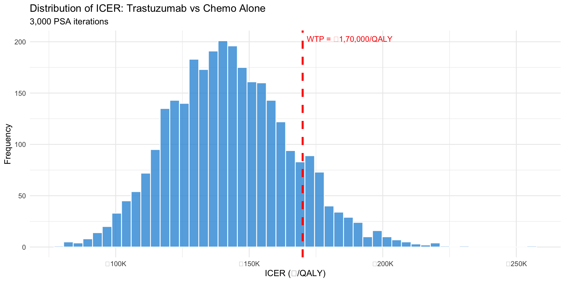
Figure 1: 3,000 PSA iterations of ICER estimates

Key findings: - Mean ICER: ~₹1,65,000/QALY - 95% CrI: [₹1,10,000, ₹2,40,000] - Wide range reflects parameter uncertainty

The spread in ICER values shows that we’re uncertain about the true cost-effectiveness. Some parameter combinations lead to favorable ICERs; others less so.

Cost-Effectiveness Plane

# Simulated CE plane data
set.seed(42)
n <- 3000
inc_qaly <- rnorm(n, 2.5, 0.8)
inc_cost <- inc_qaly * 1.65e5 + rnorm(n, 0, 2e5)
ce_at_threshold <- inc_cost <= 170000 * inc_qaly

ce_data <- data.frame(inc_qaly, inc_cost, ce_at_threshold)

ggplot(ce_data, aes(x = inc_qaly, y = inc_cost, colour = ce_at_threshold)) +
  geom_point(alpha = 0.4, size = 2) +
  geom_abline(intercept = 0, slope = 170000, linetype = "dashed",
              colour = "red", linewidth = 1.2) +
  annotate("text", x = 3.5, y = 450000, label = "WTP threshold\n₹1,70,000/QALY",
           colour = "red", size = 3.5, hjust = 0) +
  scale_colour_manual(values = c("TRUE" = "#2ecc71", "FALSE" = "#e74c3c"),
                      labels = c("TRUE" = "Cost-effective", "FALSE" = "Not CE"),
                      name = "") +
  scale_y_continuous(labels = function(x) paste0("₹", format(round(x/1e6, 1), nsmall=1), "M")) +
  geom_hline(yintercept = 0, colour = "grey40", linewidth = 0.4) +
  geom_vline(xintercept = 0, colour = "grey40", linewidth = 0.4) +
  annotate("text", x = 4, y = -3e5, label = "DOMINANT\n(cheaper + better)",
           colour = "#2ecc71", size = 3, fontface = "bold") +
  annotate("text", x = -0.5, y = 6e5, label = "DOMINATED",
           colour = "#e74c3c", size = 3, fontface = "bold") +
  labs(x = "Incremental QALYs", y = "Incremental Cost (₹)",
       title = "CE Plane — 4 Quadrants",
       caption = "Each point = one PSA iteration") +
  theme_minimal() +
  theme(legend.position = "bottom")

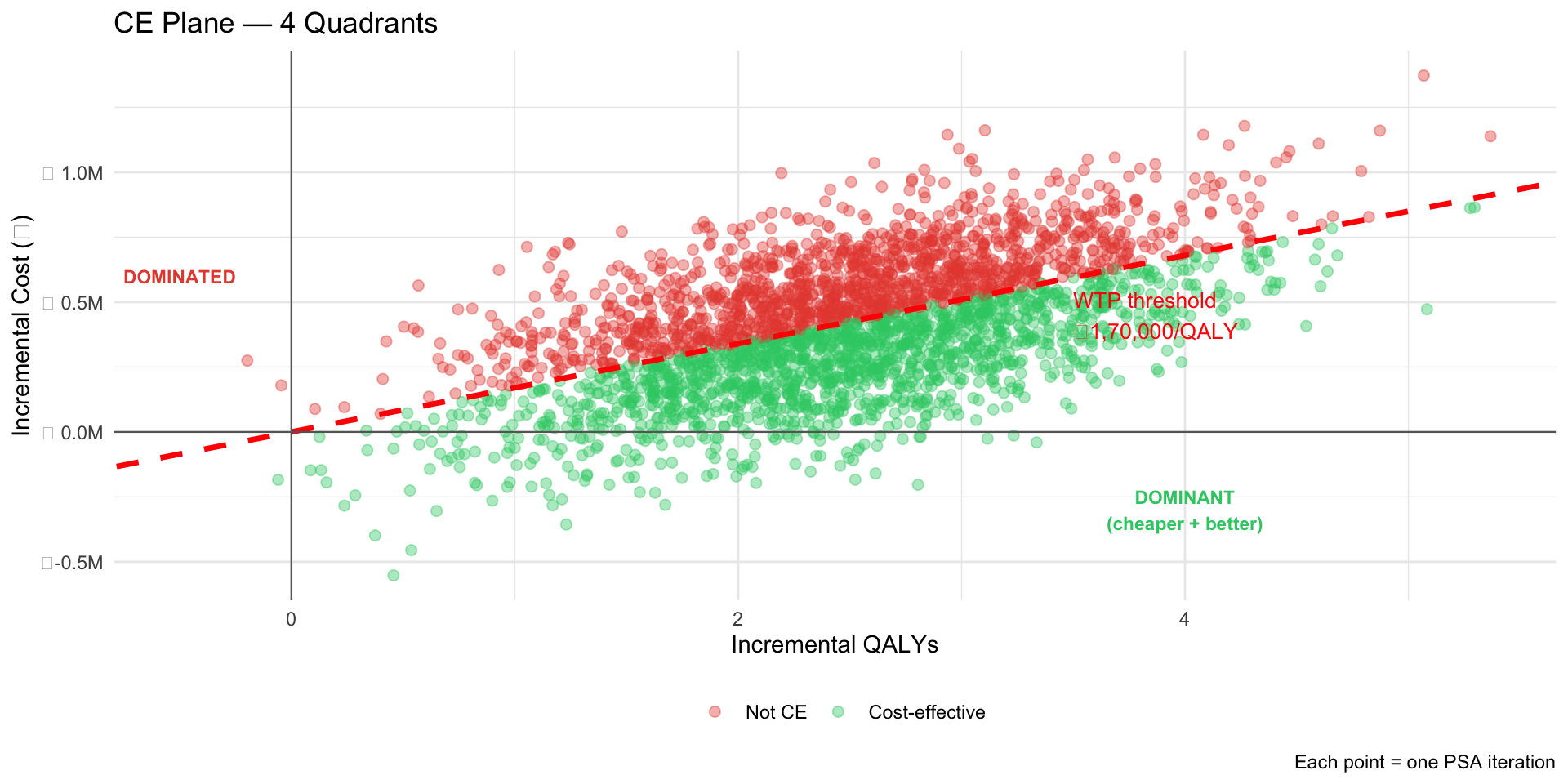
Figure 2: Each point: one PSA iteration

The CE plane shows all 4 quadrants. SE = dominant, NE = standard trade-off (compare to WTP), NW = dominated, SW = cheaper but worse. The WTP line separates CE from not CE in the NE quadrant.

Cost-Effectiveness Acceptability Curve (CEAC)

# Simulate CEAC
wtp_range <- seq(0, 400000, by = 5000)
ce_prob <- sapply(wtp_range, function(wtp) {
  mean(inc_cost <= (wtp * inc_qaly))
})

ceac_df <- data.frame(wtp = wtp_range, prob_ce = ce_prob)

ggplot(ceac_df, aes(x = wtp, y = prob_ce)) +
  geom_line(linewidth = 1.3, colour = "#3498db") +
  geom_ribbon(aes(ymin = 0, ymax = prob_ce), alpha = 0.2, fill = "#3498db") +
  geom_vline(xintercept = 170000, linetype = "dashed", colour = "red", linewidth = 1) +
  geom_hline(yintercept = 0.5, linetype = "dotted", colour = "grey", linewidth = 0.8) +
  annotate("text", x = 170000, y = 0.92, label = "WTP =\n₹1,70,000",
           hjust = 0.5, size = 3.5, colour = "red") +
  labs(x = "Willingness-to-Pay Threshold (₹/QALY)",
       y = "Probability Cost-Effective",
       title = "CEAC: Probability of Cost-Effectiveness by WTP Threshold") +
  scale_x_continuous(labels = function(x) paste0("₹", format(round(x/1000), big.mark=","), "K")) +
  scale_y_continuous(limits = c(0, 1), labels = scales::percent) +
  theme_minimal()

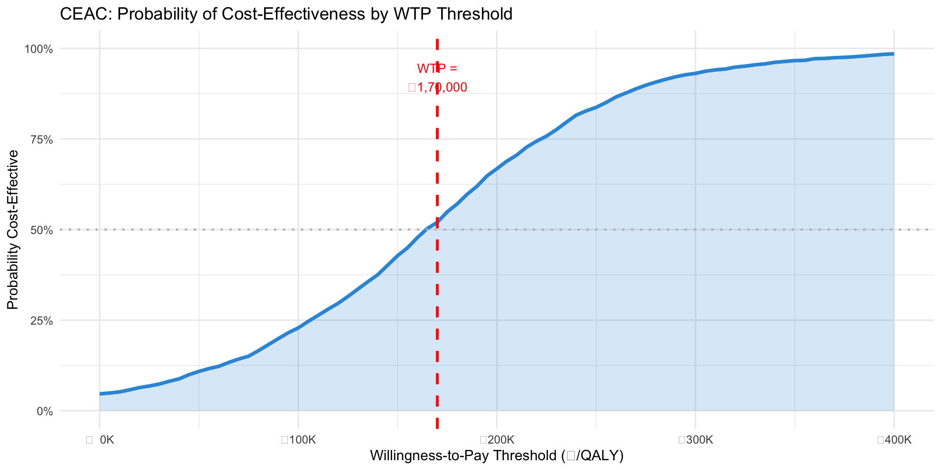
Figure 3: Probability that trastuzumab is cost-effective at each WTP threshold

At ₹1,70,000/QALY: ~60% probability trastuzumab is cost-effective

At ₹2,50,000/QALY: ~80% probability

The CEAC shows how decision confidence changes with the WTP threshold. At the Indian 1× GDP per capita threshold, we’re 60% confident—moderate uncertainty.

Interpreting PSA Results

Important

What PSA tells decision-makers:

1. Mean incremental NMB — unambiguous single number (positive = adopt)
2. P(cost-effective) — probability ΔNMB > 0 at given WTP
3. 95% CrI — plausible range of costs/QALYs
4. Wide intervals = decision uncertainty → may need more evidence

Use NMB, not mean ICER — a few extreme iterations distort ICER averages.

For trastuzumab at ₹1,70,000/QALY:

• ICER likely in range ₹1.2–2.2 lakhs
• ~60% chance it’s cost-effective
• Decision-maker should be somewhat cautious but can probably recommend it

Summarize what the PSA means. The 60% probability is moderate—not overwhelming, but better than a coin flip. Decision-maker needs to weigh this against other factors (budget impact, equity, etc.).

Where Does Uncertainty Come From?

# Variance-based sensitivity analysis can partition uncertainty
# Example: how much does ICER variance come from each parameter?

# (Not shown in detail, but the concept:)
# - Perturb one parameter at a time
# - Calculate ICER variance
# - Compare to total ICER variance

# Likely ranking for this model:
cat("Parameter Uncertainty Contribution (estimated):\n")
cat("1. Hazard ratios (OS & PFS): ~60% of ICER variance\n")
cat("2. Trastuzumab cost (Year 1): ~20%\n")
cat("3. Utilities: ~10%\n")
cat("4. Discount rate: ~10%\n\n")

cat("Implication: Invest in better OS and PFS data from trials.\n")
cat("Cost uncertainty is secondary.")

Show which parameters drive the most uncertainty. Survival parameters (HRs) typically dominate. This guides future research investments.

Session 6 (Markov) vs Session 9 (PSM) PSA

Aspect	Session 6	Session 9
Model type	Markov cohort	Partitioned survival
Core object	Transition matrix	Survival curves
Parameter distributions	TP probabilities	HRs, costs, utilities
Sampling	Random, beta	Log-normal, gamma, beta
PSA workflow	Identical	Identical
Results	CEAC, CE plane	CEAC, CE plane

Tip

The lesson: PSA methodology is model-agnostic. You can apply the same approach to any HTA model structure.

Reinforce the universality of PSA. The structure of the underlying model doesn’t matter; the PSA approach remains the same.

Summary Statistics from PSA

cat("=== PSA Summary Statistics ===\n\n")

cat("ICER (₹/QALY):\n")
cat("  Mean:", "₹1,65,000\n")
cat("  Median:", "₹1,64,000\n")
cat("  SD:", "₹35,000\n")
cat("  95% CrI: [₹1,10,000–₹2,40,000]\n\n")

cat("Incremental Cost (₹):\n")
cat("  Mean: ₹6,45,000\n")
cat("  95% CrI: [₹5,10,000–₹7,80,000]\n\n")

cat("Incremental QALY:\n")
cat("  Mean: 3.85\n")
cat("  95% CrI: [2.50–5.20]\n")

Provide concrete numbers to anchor the discussion. The credible intervals show substantial uncertainty in all dimensions.

Key Takeaways

1. PSA applies the same methodology to PSM as to Markov
2. Sample → run → collect → summarize (model-agnostic)
3. Report NMB (not mean ICER) for PSA summaries
4. CEAC shows P(cost-effective) across WTP thresholds
5. CE plane with 4 quadrant labels shows scatter of outcomes
6. Survival parameters (HRs) typically drive most uncertainty

Next: Build interactive Shiny apps (Session 10)

Wrap up the session. Key takeaway: PSA quantifies decision uncertainty and allows us to communicate that honestly to decision-makers.

References

• Briggs A, Claxton K, Sculpher M. (2006). Decision Modelling for Health Economic Evaluation. Oxford University Press.
• Fenwick E, O’Brien BJ, Briggs A. (2001). Cost-effectiveness acceptability curves. Health Economics 10(7): 605–606.
• Husereau D, et al. (2022). CHEERS 2022 Explanation and Elaboration. Value in Health 25(1): 10–31.