11  Categorical Data — Chi-square, Fisher’s, and Risk Measures

Statistical Analysis of Exposure-Disease Relationships

Lecture slides for this module: Open Slides

11.1 Learning Objectives

By the end of this module, you will be able to:

1. Construct and interpret contingency tables (2×2 and r×c) for categorical data
2. Apply chi-square test of independence and understand expected frequencies and degrees of freedom
3. Distinguish between Fisher’s exact test and Yates’ correction and when each is appropriate
4. Explain McNemar’s test for paired categorical data in before-after studies
5. Calculate and interpret measures of association: Relative Risk (RR), Odds Ratio (OR), ARR, RRR, NNT, NNH, AR, and PAR
6. Understand when OR ≈ RR and the critical difference between them at high disease prevalence
7. Develop a decision tree for choosing the correct test for categorical data analysis

---

11.2 Clinical Hook

An Outbreak Investigation in Rural Madhya Pradesh

It’s monsoon season in a village near Sagar, Madhya Pradesh. On June 15, 200 residents attend a community feast organised for a wedding. By June 17, local ASHA workers report that 80 villagers have developed acute gastroenteritis (abdominal cramps, diarrhoea, vomiting). The district surveillance officer arrives with her team.

She suspects three main dishes: biryani, paneer tikka, and samosas. She conducts a case-control study (matching 80 affected individuals with 80 unaffected attendees) and constructs 2×2 contingency tables.

For biryani exposure:

	Ate Biryani	Did Not Eat Biryani	Total
Ill	65	15	80
Well	30	50	80
Total	95	65	160

Your Tasks:

1. Was the biryani the culprit? (Chi-square test)
2. How much more likely are people who ate biryani to get sick? (Odds Ratio)
3. If you were the food safety officer, would you shut down the catering business?

By the end of this module, you’ll have the statistical tools to answer these questions with confidence.

---

11.3 Section 1: Contingency Tables and Chi-square Test

1.1 The 2×2 Contingency Table

A 2×2 contingency table organizes data where two categorical variables, each with two levels, are cross-tabulated:

X.	X..Disease..	X..No.Disease..	X..Total..
**Exposed**	a	b	a+b
**Not Exposed**	c	d	c+d
**Total**	a+c	b+d	N

Where:

• a = exposed with disease
• b = exposed without disease
• c = not exposed with disease
• d = not exposed without disease
• N = total sample size

Outbreak Data (Biryani Exposure)

X.	X..Ate.Biryani..	X..Did.Not.Eat.Biryani..	X..Total..
**Ill (Gastroenteritis)**	65	15	80
**Well**	30	50	80
**Total**	95	65	160

In our outbreak data: a = 65, b = 30, c = 15, d = 50.

---

1.2 Chi-square Test of Independence

The chi-square test determines whether two categorical variables are independent (unrelated) or associated.

Hypotheses:

• H₀: Exposure and disease are independent (not associated)
• H₁: Exposure and disease are associated (dependent)

Chi-square formula (in words): For each cell, take the difference between what you observed and what you expected under independence, square it, and divide by the expected. Sum across all cells.

\[\chi^2 = \sum \frac{(\text{Observed} - \text{Expected})^2}{\text{Expected}} = \sum \frac{(O_i - E_i)^2}{E_i}\]

Expected frequency for cell (i, j):

\[E_{ij} = \frac{(\text{Row Total}_i) \times (\text{Column Total}_j)}{\text{Grand Total}}\]

For a 2×2 table, the simplified formula is:

\[\chi^2 = \frac{N(ad - bc)^2}{(a+b)(c+d)(a+c)(b+d)}\]

Degrees of freedom: \(df = (r - 1) \times (c - 1)\). For a 2×2 table: df = 1.

---

1.3 Worked Example: Biryani Outbreak

Step 1: Calculate expected frequencies

# Observed data
a <- 65  # ill, ate biryani
b <- 30  # well, ate biryani
c <- 15  # ill, didn't eat biryani
d <- 50  # well, didn't eat biryani
N <- a + b + c + d

# Expected frequencies
E_ill_biryani     <- ((a + c) * (a + b)) / N
E_well_biryani    <- ((b + d) * (a + b)) / N
E_ill_no_biryani  <- ((a + c) * (c + d)) / N
E_well_no_biryani <- ((b + d) * (c + d)) / N

cat("Expected Frequencies:\n")

Expected Frequencies:

cat("Ill, Ate Biryani:", round(E_ill_biryani, 2), "\n")

Ill, Ate Biryani: 47.5 

cat("Well, Ate Biryani:", round(E_well_biryani, 2), "\n")

Well, Ate Biryani: 47.5 

cat("Ill, No Biryani:", round(E_ill_no_biryani, 2), "\n")

Ill, No Biryani: 32.5 

cat("Well, No Biryani:", round(E_well_no_biryani, 2), "\n")

Well, No Biryani: 32.5 

Step 2: Calculate chi-square statistic

chi_sq <- (N * (a*d - b*c)^2) / ((a+b) * (c+d) * (a+c) * (b+d))

cat("Chi-square statistic:", round(chi_sq, 4), "\n")

Chi-square statistic: 31.7409 

cat("Degrees of freedom: 1\n")

Degrees of freedom: 1

p_value <- 1 - pchisq(chi_sq, df = 1)
cat("p-value:", format(p_value, scientific = TRUE), "\n")

p-value: 1.761736e-08 

cat("\nInterpretation: p < 0.05, so we REJECT H₀.\n")

Interpretation: p < 0.05, so we REJECT H₀.

cat("The biryani exposure and illness ARE significantly associated.\n")

The biryani exposure and illness ARE significantly associated.

Key Insight

A small p-value (< 0.05) indicates that the observed pattern is unlikely under the assumption of independence. This strongly suggests that eating biryani and developing gastroenteritis are not independent — the biryani is likely the culprit.

---

1.4 Visualising the Outbreak Data

# Create contingency table
outbreak_table <- matrix(c(65, 30, 15, 50), nrow = 2, byrow = TRUE)
dimnames(outbreak_table) <- list(
  Biryani = c("Ate", "Did Not Eat"),
  Health = c("Ill", "Well")
)

# Mosaic plot
mosaic(outbreak_table,
       shade = TRUE,
       legend = TRUE,
       main = "Biryani Exposure and Gastroenteritis\nOutbreak Investigation, Sagar District",
       xlab = "Biryani Exposure",
       ylab = "Health Outcome",
       gp = shading_Friendly)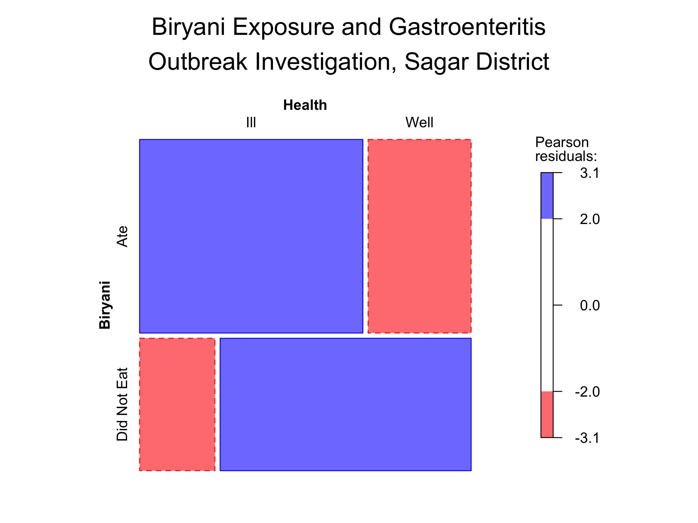

The size of each rectangle represents the proportion of people in that category. The shading indicates whether the observed count is more (blue) or less (red) than expected under independence.

1.5 Observed vs. Expected Frequencies

freq_data <- data.frame(
  Category = c("Ate Biryani, Ill", "Ate Biryani, Well",
               "No Biryani, Ill", "No Biryani, Well"),
  Observed = c(65, 30, 15, 50),
  Expected = c(round(E_ill_biryani, 1), round(E_well_biryani, 1),
               round(E_ill_no_biryani, 1), round(E_well_no_biryani, 1))
)

freq_long <- freq_data %>%
  pivot_longer(cols = c("Observed", "Expected"),
               names_to = "Type", values_to = "Frequency")

ggplot(freq_long, aes(x = Category, y = Frequency, fill = Type)) +
  geom_col(position = "dodge", alpha = 0.8) +
  geom_text(aes(label = round(Frequency, 1)),
            position = position_dodge(width = 0.9), vjust = -0.5) +
  labs(title = "Observed vs. Expected Frequencies",
       subtitle = "Biryani outbreak 2×2 table",
       x = "Category", y = "Frequency",
       fill = "Frequency Type") +
  theme_clean() +
  theme(axis.text.x = element_text(angle = 45, hjust = 1, size = 10))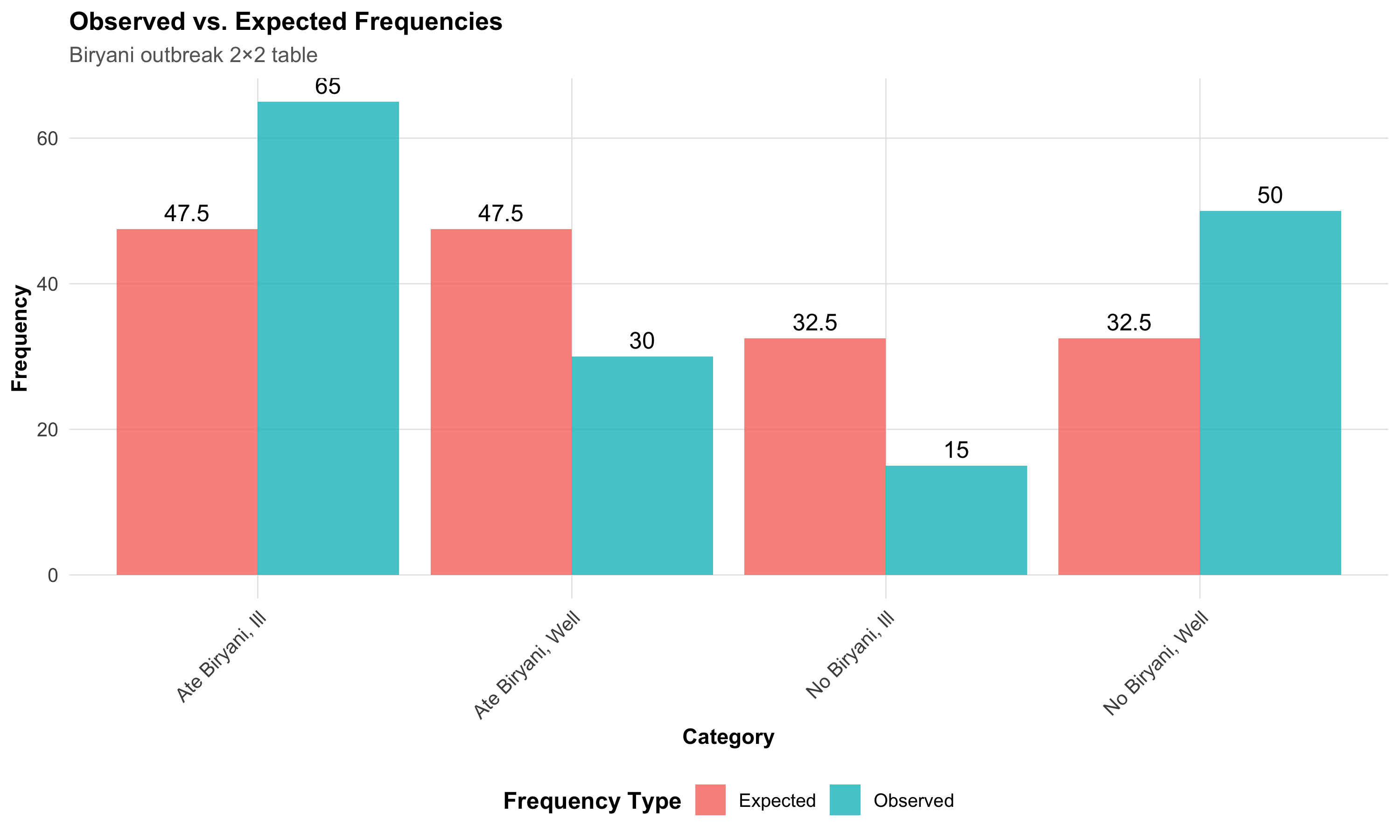

The Chi-square Formula at a Glance

For a 2×2 table:

\[\chi^2 = \frac{N(ad - bc)^2}{(a+b)(c+d)(a+c)(b+d)}\]

The numerator is the cross-product difference. The larger the discrepancy between \(ad\) and \(bc\), the larger chi-square, and the stronger the evidence against independence.

---

11.4 Section 2: Assumptions and Alternatives

2.1 Assumptions of the Chi-square Test

The chi-square test requires:

1. Random sample from the population
2. Independence of observations (each person counted only once)
3. Adequate sample size — all expected frequencies ≥ 5 (for a 2×2 table)

When these assumptions are violated, we turn to alternatives.

---

2.2 Fisher’s Exact Test

When expected cell frequency < 5 in any cell of a 2×2 table, use Fisher’s exact test. It computes exact probabilities rather than relying on the chi-square approximation.

When to use Fisher’s:

• Any expected frequency < 5 in a 2×2 table
• Small sample sizes (N < 20–30)
• Rare diseases or rare exposures

Worked example: A small cluster of leptospirosis cases after flooding in Alappuzha, Kerala. Only 25 individuals are studied:

small_outbreak <- matrix(c(8, 2, 3, 12), nrow = 2, byrow = TRUE)
dimnames(small_outbreak) <- list(
  Exposure = c("Waded in floodwater", "Did not wade"),
  Disease = c("Leptospirosis", "Healthy")
)

cat("Small Outbreak 2×2 Table:\n")

Small Outbreak 2×2 Table:

print(small_outbreak)

                     Disease
Exposure              Leptospirosis Healthy
  Waded in floodwater             8       2
  Did not wade                    3      12

cat("\n")

fisher_result <- fisher.test(small_outbreak)
cat("Fisher's Exact Test Results:\n")

Fisher's Exact Test Results:

cat("p-value:", round(fisher_result$p.value, 4), "\n")

p-value: 0.0051 

cat("Odds Ratio:", round(fisher_result$estimate, 2), "\n")

Odds Ratio: 13.77 

Common Mistake

Using chi-square when expected frequencies are < 5. The p-value becomes unreliable. Always check expected frequencies first.

Rule of thumb: For a 2×2 table with N < 30 or any expected frequency < 5, default to Fisher’s exact test.

---

2.3 Yates’ Continuity Correction

For moderate sample sizes (20 < N < 50), some texts recommend Yates’ correction:

\[\chi^2_{\text{Yates}} = \frac{N(|ad - bc| - N/2)^2}{(a+b)(c+d)(a+c)(b+d)}\]

Modern perspective: Yates’ correction is often considered overly conservative and not routinely recommended. Fisher’s exact test is preferred for small samples, and the standard chi-square is fine for large samples.

---

2.4 McNemar’s Test for Paired Categorical Data

When the same subjects are measured twice (before–after or paired design), use McNemar’s test.

Scenario: A TB control programme in Patna, Bihar, tests 100 contacts of TB patients for knowledge about transmission — before and after a health education session.

The McNemar table records who changed their answer:

	After: Correct	After: Incorrect
Before: Correct	55 (concordant)	5 (lost knowledge)
Before: Incorrect	25 (gained knowledge)	15 (concordant)

Only the discordant pairs (b = 5, c = 25) contribute to the test:

\[\chi^2_{\text{McNemar}} = \frac{(b - c)^2}{b + c}\]

b <- 5   # Before correct, After incorrect
c <- 25  # Before incorrect, After correct

chi_sq_mcnemar <- (b - c)^2 / (b + c)
p_mcnemar <- 1 - pchisq(chi_sq_mcnemar, df = 1)

cat("McNemar's Test for TB Health Education Programme\n")

McNemar's Test for TB Health Education Programme

cat("Discordant pairs: b =", b, ", c =", c, "\n")

Discordant pairs: b = 5 , c = 25 

cat("Chi-square statistic:", round(chi_sq_mcnemar, 4), "\n")

Chi-square statistic: 13.3333 

cat("p-value:", round(p_mcnemar, 4), "\n")

p-value: 3e-04 

cat("\nThe proportion with correct knowledge significantly\n")

The proportion with correct knowledge significantly

cat("increased after health education (p < 0.05).\n")

increased after health education (p < 0.05).

McNemar’s Test

Use when comparing paired categorical outcomes (same subject, before–after). It is the categorical equivalent of the paired t-test. Concordant pairs are ignored — only those who changed contribute to the test statistic.

---

11.5 Section 3: Measures of Association

We move beyond “is there an association?” to “how strong is the association?” and “what is the clinical impact?”

3.1 Risk and Probability

From a 2×2 table:

• Risk in Exposed: \(P(\text{Disease | Exposed}) = \frac{a}{a+b}\)
• Risk in Unexposed: \(P(\text{Disease | Unexposed}) = \frac{c}{c+d}\)

# Reset outbreak data
a <- 65; b <- 30; c <- 15; d <- 50

risk_exposed   <- a / (a + b)
risk_unexposed <- c / (c + d)
cat("Risk in Exposed (ate biryani):", round(risk_exposed, 3),
    paste0("(", round(risk_exposed * 100, 1), "%)"), "\n")

Risk in Exposed (ate biryani): 0.684 (68.4%) 

cat("Risk in Unexposed (no biryani):", round(risk_unexposed, 3),
    paste0("(", round(risk_unexposed * 100, 1), "%)"), "\n")

Risk in Unexposed (no biryani): 0.231 (23.1%) 

---

3.2 Relative Risk (RR)

Relative Risk compares disease incidence between exposed and unexposed groups.

In words:

\[RR = \frac{\text{Risk of disease in Exposed}}{\text{Risk of disease in Unexposed}}\]

In cell notation:

\[RR = \frac{a/(a+b)}{c/(c+d)}\]

Interpretation: RR = 1 means no association; RR > 1 means increased risk; RR < 1 means protective.

RR <- risk_exposed / risk_unexposed
cat("Relative Risk (RR):", round(RR, 3), "\n")

Relative Risk (RR): 2.965 

cat("\nPeople who ate biryani were", round(RR, 1), "times more likely\n")

People who ate biryani were 3 times more likely

cat("to develop gastroenteritis compared to those who didn't.\n")

to develop gastroenteritis compared to those who didn't.

Relative Risk (RR)

\[RR = \frac{\text{Incidence in Exposed}}{\text{Incidence in Unexposed}} = \frac{a/(a+b)}{c/(c+d)}\]

Used in: Cohort studies (follow exposed and unexposed groups forward in time).

Advantage: Directly estimates the factor by which risk changes with exposure.

Limitation: Can only be calculated from cohort studies where you can compute incidence; case-control studies must use the Odds Ratio.

---

3.3 Odds Ratio (OR)

The odds of disease given exposure = number with disease divided by number without disease in the exposed group = \(a/b\).

In words:

\[OR = \frac{\text{Odds of disease in Exposed}}{\text{Odds of disease in Unexposed}}\]

In cell notation (two equivalent forms):

\[OR = \frac{a/b}{c/d} = \frac{ad}{bc} \quad \text{(cross-product ratio)}\]

The cross-product form (\(ad/bc\)) is the quickest way to compute OR from a 2×2 table — multiply the diagonal cells and take the ratio.

odds_exposed   <- a / b
odds_unexposed <- c / d
OR <- odds_exposed / odds_unexposed

cat("Odds of illness in exposed:", round(odds_exposed, 3), "\n")

Odds of illness in exposed: 2.167 

cat("Odds of illness in unexposed:", round(odds_unexposed, 3), "\n")

Odds of illness in unexposed: 0.3 

cat("\nOdds Ratio (OR):", round(OR, 3), "\n")

Odds Ratio (OR): 7.222 

cat("\nThe odds of gastroenteritis are", round(OR, 2),
    "times higher\nin those who ate biryani.\n")

The odds of gastroenteritis are 7.22 times higher
in those who ate biryani.

---

3.4 When Does OR ≈ RR? The Critical Relationship

NEET PG High-Yield

\[OR \approx RR \text{ when disease is RARE (incidence < 5–10%)}\]

When disease is common (incidence > 20%), OR greatly overestimates RR.

scenarios <- expand_grid(
  Prevalence = c(0.01, 0.05, 0.10, 0.20, 0.40),
  RR = c(1.5, 2.0, 3.0)
)

scenarios <- scenarios %>%
  mutate(
    baseline_risk = Prevalence,
    risk_exposed = baseline_risk * RR,
    OR_est = RR * ((1 - baseline_risk) / (1 - risk_exposed))
  ) %>%
  select(Prevalence, RR, OR_est) %>%
  mutate(
    across(c(Prevalence, OR_est), ~ round(., 3)),
    Prevalence = paste0(Prevalence * 100, "%")
  ) %>%
  arrange(desc(Prevalence))

kable(scenarios, col.names = c("Disease Prevalence", "Relative Risk", "Odds Ratio (Est.)"),
      format = "html") %>%
  kable_styling(full_width = FALSE, bootstrap_options = c("bordered", "hover")) %>%
  row_spec(0, bold = TRUE, background = "#D3D3D3")

Disease Prevalence	Relative Risk	Odds Ratio (Est.)
5%	1.5	1.541
5%	2.0	2.111
5%	3.0	3.353
40%	1.5	2.250
40%	2.0	6.000
40%	3.0	-9.000
20%	1.5	1.714
20%	2.0	2.667
20%	3.0	6.000
10%	1.5	1.588
10%	2.0	2.250
10%	3.0	3.857
1%	1.5	1.508
1%	2.0	2.020
1%	3.0	3.062

At 1% prevalence the OR closely matches the RR. At 40% prevalence the OR overshoots by 50% or more.

prev_range <- seq(0.01, 0.60, by = 0.02)
rr_val <- 2.5

or_vals <- rr_val * ((1 - prev_range) / (1 - prev_range * rr_val))

df_or_rr <- data.frame(
  Prevalence = prev_range * 100,
  RR = rr_val,
  OR = or_vals
) %>%
  pivot_longer(cols = c("RR", "OR"), names_to = "Measure", values_to = "Value")

ggplot(df_or_rr, aes(x = Prevalence, y = Value, color = Measure,
                      linetype = Measure)) +
  geom_line(linewidth = 1.2) +
  geom_hline(yintercept = rr_val, linetype = "dashed", color = "gray",
             linewidth = 0.5) +
  scale_color_manual(values = c("RR" = "#1f77b4", "OR" = "#ff7f0e")) +
  scale_linetype_manual(values = c("RR" = "solid", "OR" = "dashed")) +
  annotate("text", x = 35, y = rr_val + 0.2, label = "RR constant = 2.5",
           color = "#1f77b4", fontface = "bold") +
  annotate("text", x = 50, y = 5, label = "OR diverges\nfrom RR at\nhigh prevalence",
           color = "#ff7f0e", fontface = "bold") +
  labs(title = "Odds Ratio vs. Relative Risk",
       subtitle = "RR = 2.5 fixed; disease prevalence varies",
       x = "Disease Prevalence (%)",
       y = "Measure Value") +
  theme_clean()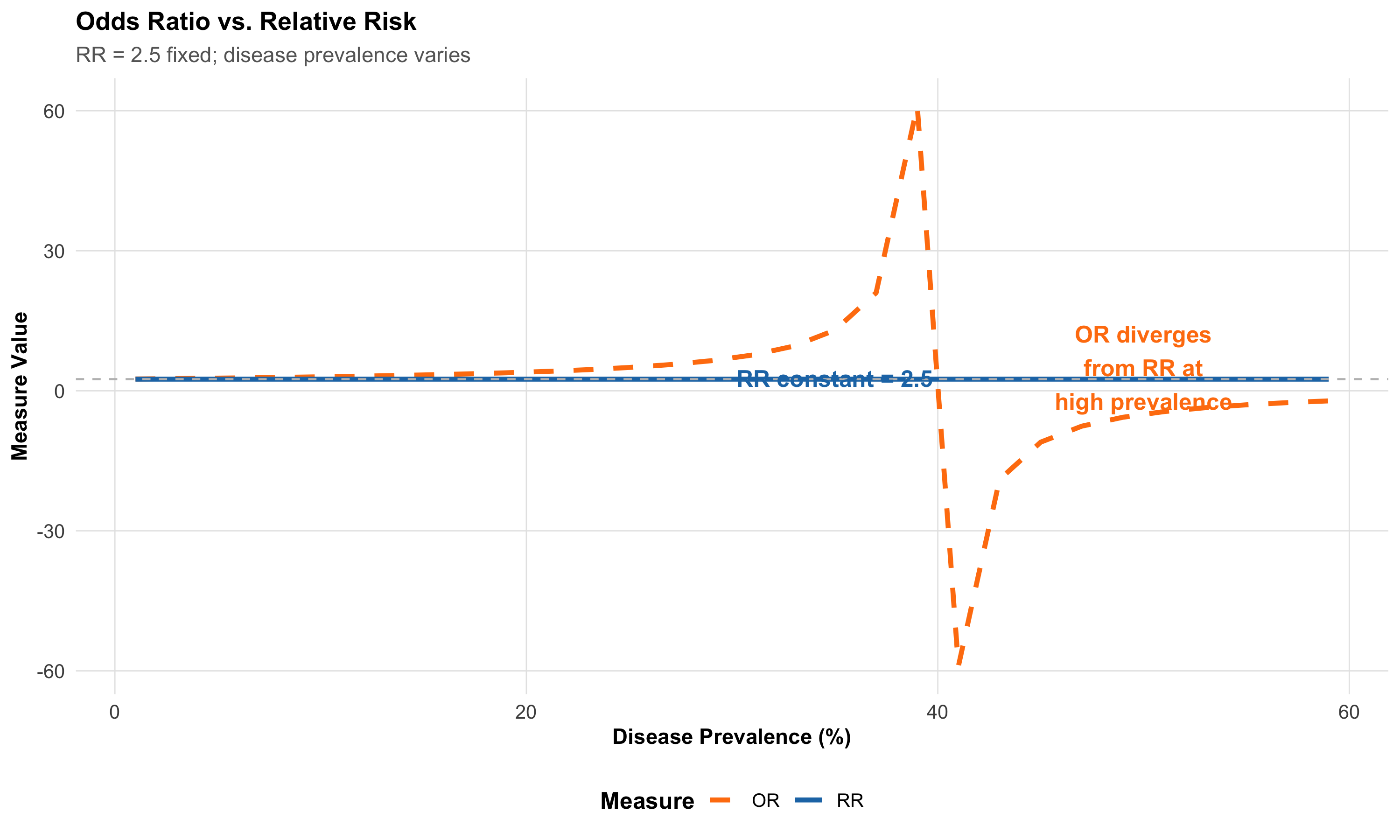

NEET PG Trap

A case-control study of melanoma reports OR = 3.2 for sun exposure. A student incorrectly states: “Sun exposure increases melanoma risk by 3.2 times.”

The error: Case-control studies cannot directly estimate RR. The OR = 3.2 approximates RR only if melanoma is rare. If prevalence is high, OR overestimates the true RR.

Correct statement: “The odds of past sun exposure are 3.2 times higher in cases than controls. Under the rare disease assumption, RR ≈ 3.2.”

---

3.5 Confidence Intervals for OR

\[OR_{95\%CI} = OR \times e^{\pm 1.96 \times SE(\ln OR)}\]

where \(SE(\ln OR) = \sqrt{\frac{1}{a} + \frac{1}{b} + \frac{1}{c} + \frac{1}{d}}\)

ln_OR <- log(OR)
se_ln_OR <- sqrt(1/a + 1/b + 1/c + 1/d)
margin_error <- 1.96 * se_ln_OR

or_ci_lower <- exp(ln_OR - margin_error)
or_ci_upper <- exp(ln_OR + margin_error)

cat("Odds Ratio and 95% Confidence Interval:\n")

Odds Ratio and 95% Confidence Interval:

cat("OR =", round(OR, 3), "\n")

OR = 7.222 

cat("95% CI:", round(or_ci_lower, 3), "–", round(or_ci_upper, 3), "\n")

95% CI: 3.511 – 14.855 

cat("\nSince the CI does NOT include 1.0, the association\n")

Since the CI does NOT include 1.0, the association

cat("is statistically significant at the 0.05 level.\n")

is statistically significant at the 0.05 level.

Confidence Interval Rule

• CI includes 1.0: Not statistically significant (p > 0.05)
• CI excludes 1.0: Statistically significant (p < 0.05)

---

11.6 Section 4: Measures of Impact and Clinical Significance

We shift from association (RR, OR) to impact measures that directly inform clinical decisions.

4.1 Absolute Risk Reduction (ARR) and Relative Risk Reduction (RRR)

These measures translate association into clinical impact.

In words:

• ARR = How much does treatment lower the absolute risk? = Risk in Control group − Risk in Treatment group
• RRR = What fraction of the baseline risk is removed by treatment? = ARR ÷ Risk in Control group

Scenario: A TB vaccine trial conducted across PHCs in Varanasi, Uttar Pradesh — 500 vaccinated vs. 500 unvaccinated individuals:

• Unvaccinated: 20/500 developed TB (4.0%)
• Vaccinated: 5/500 developed TB (1.0%)

risk_control       <- 20 / 500
risk_intervention  <- 5 / 500

ARR <- risk_control - risk_intervention
RRR <- ARR / risk_control

cat("Risk in Unvaccinated:", round(risk_control * 100, 2), "%\n")

Risk in Unvaccinated: 4 %

cat("Risk in Vaccinated:", round(risk_intervention * 100, 2), "%\n")

Risk in Vaccinated: 1 %

cat("\nAbsolute Risk Reduction (ARR):", round(ARR * 100, 2), "%\n")

Absolute Risk Reduction (ARR): 3 %

cat("Vaccinating prevents illness in 3 per 100 people.\n")

Vaccinating prevents illness in 3 per 100 people.

cat("\nRelative Risk Reduction (RRR):", round(RRR * 100, 2), "%\n")

Relative Risk Reduction (RRR): 75 %

cat("Vaccination reduces TB risk by 75% relative to baseline.\n")

Vaccination reduces TB risk by 75% relative to baseline.

ARR vs. RRR

\[ARR = \text{Risk}_{\text{Control}} - \text{Risk}_{\text{Intervention}}\]

\[RRR = \frac{ARR}{\text{Risk}_{\text{Control}}}\]

Critical difference: ARR is what matters clinically; RRR can sound impressive but overstate impact when baseline risk is low.

Example: If baseline risk is 1%, an intervention that halves it gives RRR = 50% (sounds great) but ARR = 0.5% (modest impact).

---

4.2 Number Needed to Treat (NNT)

NNT = how many patients you must treat to prevent one adverse outcome.

In words: If the ARR is 3% (i.e., treatment prevents disease in 3 out of every 100), then you need to treat 100/3 ≈ 33 people to prevent one case.

\[NNT = \frac{1}{ARR}\]

NNT <- 1 / ARR
cat("Number Needed to Treat (NNT):", round(NNT, 1), "\n")

Number Needed to Treat (NNT): 33.3 

cat("\nYou must vaccinate", round(NNT, 1),
    "people to prevent one case of TB.\n")

You must vaccinate 33.3 people to prevent one case of TB.

nnt_value <- round(NNT, 0)

icon_data <- data.frame(
  x = rep(1:nnt_value, length.out = nnt_value),
  y = rep(1, nnt_value),
  Status = c("Protected by vaccine", rep("No change", nnt_value - 1))
)

ggplot(icon_data, aes(x = x, y = y, fill = Status)) +
  geom_tile(color = "white", linewidth = 0.8, height = 0.8) +
  scale_fill_manual(values = c("Protected by vaccine" = "#2ecc71",
                                "No change" = "#bdc3c7")) +
  coord_equal() +
  labs(title = paste0("NNT = ", nnt_value,
                      " — Vaccinate ", nnt_value,
                      " to prevent 1 case of TB"),
       x = "", y = "", fill = "Outcome") +
  theme_void() +
  theme(plot.title = element_text(hjust = 0.5, face = "bold", size = 13),
        legend.position = "bottom")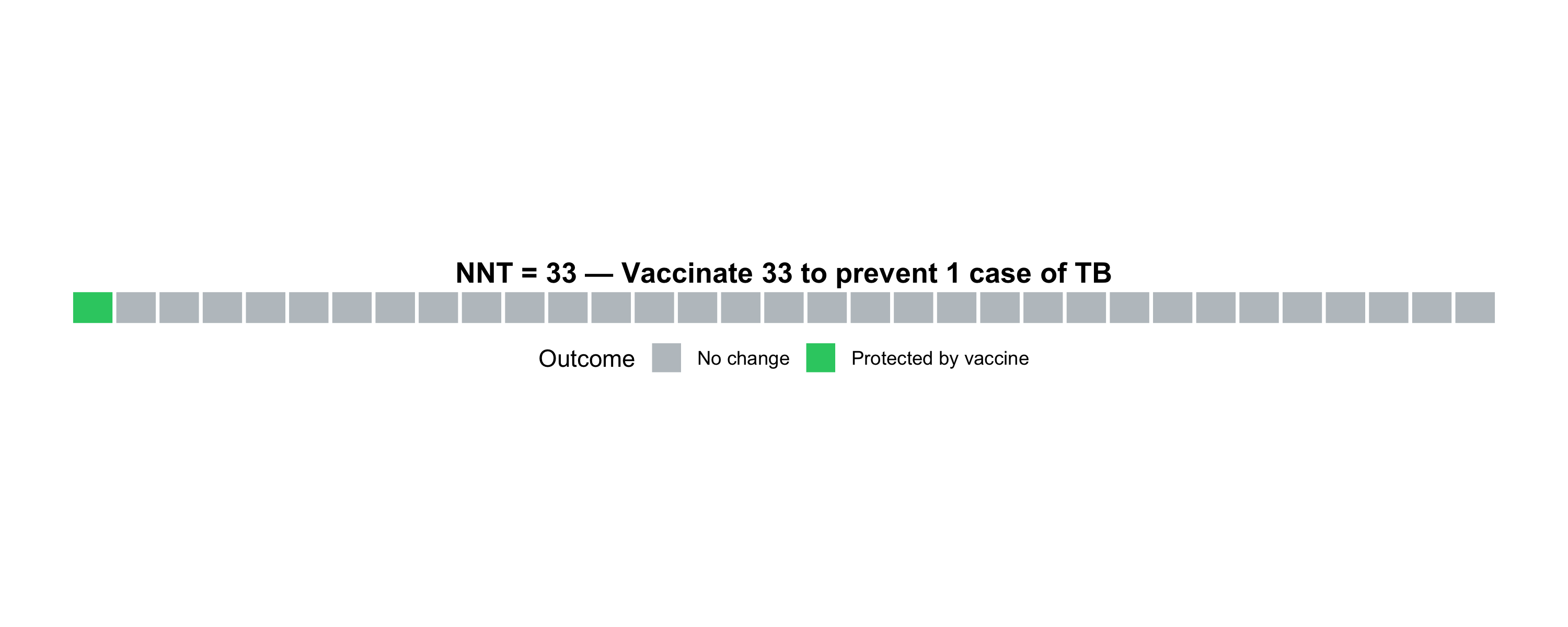

Interpreting NNT

• NNT ≈ 10: Excellent (treat 10 to save one)
• NNT ≈ 50: Moderate benefit
• NNT > 200: Modest benefit

Compare across interventions: an NNT of 15 is superior to an NNT of 40.

---

4.3 Number Needed to Harm (NNH)

\[NNH = \frac{1}{\text{Risk}_{\text{Treatment}}^{\text{harm}} - \text{Risk}_{\text{Control}}^{\text{harm}}}\]

Suppose in the same vaccine trial, severe local reactions occur in 8/500 vaccinated vs. 2/500 unvaccinated:

risk_harm_vaccine  <- 8 / 500
risk_harm_control  <- 2 / 500

ARH <- risk_harm_vaccine - risk_harm_control
NNH <- 1 / ARH

cat("Risk of severe reaction in Vaccinated:", round(risk_harm_vaccine * 100, 2), "%\n")

Risk of severe reaction in Vaccinated: 1.6 %

cat("Risk of severe reaction in Unvaccinated:", round(risk_harm_control * 100, 2), "%\n")

Risk of severe reaction in Unvaccinated: 0.4 %

cat("Absolute Risk of Harm:", round(ARH * 100, 2), "%\n")

Absolute Risk of Harm: 1.2 %

cat("\nNNH:", round(NNH, 1), "\n")

NNH: 83.3 

cat("For every", round(NNH, 0), "vaccinated, 1 has a severe reaction.\n")

For every 83 vaccinated, 1 has a severe reaction.

Therapeutic index: NNH / NNT tells you how the benefit compares to harm:

TI <- NNH / NNT
cat("Therapeutic Index (NNH/NNT):", round(TI, 2), "\n")

Therapeutic Index (NNH/NNT): 2.5 

if (TI > 1) {
  cat("Benefit clearly outweighs harm — VACCINATION RECOMMENDED.\n")
} else {
  cat("Harm exceeds benefit — reconsider intervention.\n")
}

Benefit clearly outweighs harm — VACCINATION RECOMMENDED.

---

4.4 Attributable Risk (AR) and Population Attributable Risk (PAR)

Attributable Risk (AR) answers: “How much extra disease does the exposure cause in exposed individuals?”

In words:

• AR = Risk in Exposed − Risk in Unexposed (the excess risk attributable to the exposure)
• AR% = What percentage of disease among the exposed is caused by the exposure? = (AR ÷ Risk in Exposed) × 100

Population Attributable Risk (PAR) answers: “If we could eliminate the exposure entirely, what fraction of disease in the whole population would disappear?”

• PAR depends on both the strength of association (RR) and how common the exposure is in the population (\(P_e\))

Scenario: A cohort study of smoking and lung cancer:

• Risk in smokers: 8%
• Risk in non-smokers: 1%

risk_smokers    <- 0.08
risk_nonsmokers <- 0.01

AR <- risk_smokers - risk_nonsmokers
AR_percent <- (AR / risk_smokers) * 100

cat("Attributable Risk (AR):", round(AR * 100, 2), "%\n")

Attributable Risk (AR): 7 %

cat("AR%:", round(AR_percent, 1), "%\n")

AR%: 87.5 %

cat("\n", round(AR_percent, 1), "% of lung cancer in smokers\n")

 87.5 % of lung cancer in smokers

cat("is attributable to (caused by) smoking.\n")

is attributable to (caused by) smoking.

Population Attributable Risk (PAR) answers: “What proportion of disease in the entire population is due to this exposure?”

\[PAR\% = \frac{P_e(RR - 1)}{P_e(RR - 1) + 1} \times 100\]

where \(P_e\) = prevalence of exposure.

P_e <- 0.40  # 40% of population smokes
RR_smoking <- risk_smokers / risk_nonsmokers

PAR_percent <- (P_e * (RR_smoking - 1)) / (P_e * (RR_smoking - 1) + 1) * 100

cat("Smoking prevalence:", P_e * 100, "%\n")

Smoking prevalence: 40 %

cat("RR:", round(RR_smoking, 2), "\n")

RR: 8 

cat("\nPAR%:", round(PAR_percent, 1), "%\n")

PAR%: 73.7 %

cat(round(PAR_percent, 1), "% of ALL lung cancer in the population\n")

73.7 % of ALL lung cancer in the population

cat("could be prevented if smoking were eliminated.\n")

could be prevented if smoking were eliminated.

AR vs. PAR — Clinical vs. Public Health

\[AR = \text{Risk}_{\text{Exposed}} - \text{Risk}_{\text{Unexposed}}\]

\[PAR\% = \frac{P_e(RR - 1)}{P_e(RR - 1) + 1} \times 100\]

• AR: Relevant for individual patient counselling (“your personal risk from this exposure”)
• PAR%: Relevant for public health policy (“population-level benefit of removing exposure”)

---

11.7 Section 5: Decision Guide for Test Selection

Scenario	Test / Measure	Key Note
Two independent groups, all expected freq ≥ 5	Chi-square test	Most common; requires adequate sample size
Two independent groups, any expected freq	Fisher's exact test	Exact probability; no sample size restriction
Paired / before–after categorical data	McNemar's test	Uses only discordant pairs
Ordered categories, testing for trend	Chi-square test for trend	Extension for ordinal categories
Cohort study, 2×2 table	Relative Risk (RR)	Direct risk measure; OR ≈ RR when disease is rare
Case-control study, 2×2 table	Odds Ratio (OR)	Only valid measure from case-control design
Measuring clinical impact of treatment	ARR, RRR, NNT, NNH	Translate statistical results into clinical decisions

Quick Reference Table

Study Design / Question	Test / Measure	Null Hypothesis / Assumption
Are two categorical variables associated?	Chi-square test	Variables are independent
Small sample / expected freq	Fisher's exact test	Variables are independent (exact)
Same subjects, before–after?	McNemar's test	No change in paired proportions
Cohort study (can calculate incidence)?	Relative Risk (RR)	RR = 1
Case-control study?	Odds Ratio (OR)	OR = 1
How many to treat to prevent one outcome?	NNT = 1/ARR	ARR = 0 (no benefit)
Proportion of disease due to exposure?	Attributable Risk (AR)	Risk same in exposed/unexposed
Population benefit of removing exposure?	Population Attributable Risk (PAR)	Population at baseline unexposed risk

Core Formulae — In Words and Notation

Measure	In Words	Cell Notation
Chi-square	Sum of (Observed − Expected)² ÷ Expected	\(\sum (O - E)^2 / E\)
RR	Risk in Exposed ÷ Risk in Unexposed	\(\frac{a/(a+b)}{c/(c+d)}\)
OR	Odds in Exposed ÷ Odds in Unexposed = Cross-product ratio	\(\frac{ad}{bc}\)
ARR	Risk in Control − Risk in Treatment	\(R_c - R_t\)
RRR	ARR ÷ Risk in Control	\(ARR / R_c\)
NNT	1 ÷ ARR (how many to treat to save one)	\(1 / ARR\)
NNH	1 ÷ Absolute Risk of Harm	\(1 / ARH\)
AR	Risk in Exposed − Risk in Unexposed (excess risk from exposure)	\(R_e - R_u\)
AR%	(AR ÷ Risk in Exposed) × 100	\((AR / R_e) \times 100\)
PAR%	Fraction of disease in population attributable to exposure	\(\frac{P_e(RR-1)}{P_e(RR-1)+1} \times 100\)

---

11.8 Section 6: Complete R Workflow

# ==========================================
# COMPLETE OUTBREAK ANALYSIS WORKFLOW
# ==========================================

# Step 1: Input data
a <- 65; b <- 30; c <- 15; d <- 50
N <- a + b + c + d

outbreak <- data.frame(
  Exposure = c("Ate Biryani", "Ate Biryani", "No Biryani", "No Biryani"),
  Health = c("Ill", "Well", "Ill", "Well"),
  Count = c(a, b, c, d)
)

cont_table <- xtabs(Count ~ Exposure + Health, data = outbreak)
print(cont_table)

             Health
Exposure      Ill Well
  Ate Biryani  65   30
  No Biryani   15   50

# Step 2: Chi-square test
chi_test <- chisq.test(cont_table)
cat("\n--- CHI-SQUARE TEST ---\n")

--- CHI-SQUARE TEST ---

print(chi_test)

    Pearson's Chi-squared test with Yates' continuity correction

data:  cont_table
X-squared = 29.953, df = 1, p-value = 4.426e-08

# Step 3: Measures of association
risk_exp   <- a / (a + b)
risk_unexp <- c / (c + d)
RR <- risk_exp / risk_unexp
OR <- (a * d) / (b * c)

ln_OR    <- log(OR)
se_ln_OR <- sqrt(1/a + 1/b + 1/c + 1/d)
or_ci    <- exp(ln_OR + c(-1, 1) * 1.96 * se_ln_OR)

ARR <- risk_exp - risk_unexp

cat("\n--- MEASURES OF ASSOCIATION ---\n")

--- MEASURES OF ASSOCIATION ---

cat("Risk in Exposed:", round(risk_exp, 3), "\n")

Risk in Exposed: 0.684 

cat("Risk in Unexposed:", round(risk_unexp, 3), "\n")

Risk in Unexposed: 0.231 

cat("Relative Risk (RR):", round(RR, 3), "\n")

Relative Risk (RR): 2.965 

cat("Odds Ratio (OR):", round(OR, 3), "\n")

Odds Ratio (OR): 7.222 

cat("95% CI for OR:", round(or_ci[1], 3), "–", round(or_ci[2], 3), "\n")

95% CI for OR: 3.511 – 14.855 

cat("ARR:", round(ARR * 100, 2), "%\n")

ARR: 45.34 %

cat("\n--- INTERPRETATION ---\n")

--- INTERPRETATION ---

cat("Biryani exposure is significantly associated with\n")

Biryani exposure is significantly associated with

cat("gastroenteritis (χ² =", round(chi_test$statistic, 3),
    ", p =", round(chi_test$p.value, 4), ").\n")

gastroenteritis (χ² = 29.953 , p = 0 ).

cat("People eating biryani were", round(RR, 1),
    "times more likely to get ill.\n")

People eating biryani were 3 times more likely to get ill.

cat("The odds of illness were", round(OR, 1),
    "times higher in those who ate biryani.\n")

The odds of illness were 7.2 times higher in those who ate biryani.

---

11.9 Summary

Key Takeaways

1. Chi-square test determines whether two categorical variables are associated. Check expected frequencies ≥ 5; use Fisher’s exact test for small samples.

2. McNemar’s test handles paired categorical data (before–after). It only uses discordant pairs.

3. Relative Risk (RR) compares incidence in exposed vs. unexposed — used in cohort studies.

4. Odds Ratio (OR) compares odds — used in case-control studies. When disease is rare (< 5–10%), OR ≈ RR. At high prevalence, OR overestimates RR.

5. NNT = 1/ARR answers “How many must I treat to prevent one outcome?” Lower NNT = greater benefit.

6. AR and PAR quantify individual and population-level impact, guiding public health policy.

7. Always report 95% CI for OR and RR. If the CI excludes 1.0, the result is statistically significant.

---

11.10 Practice Questions

Q1: Number Needed to Treat

A vaccine trial enrolls 500 vaccinated and 500 unvaccinated individuals. Over 2 years, 10 vaccinated and 40 unvaccinated develop typhoid. What is the NNT?

A. 6.7 B. 16.7 C. 12.5 D. 25.0

✘ A. 6.7 — Incorrect. This uses the wrong denominator — check your ARR calculation.

✔ B. 16.7 — Correct! ARR = 40/500 − 10/500 = 0.06. NNT = 1/0.06 = 16.7. About 17 people must be vaccinated to prevent one case.

✘ C. 12.5 — Incorrect. This confuses the ARR with a different quantity.

✘ D. 25.0 — Incorrect. This is 1/(risk in unvaccinated), not 1/ARR.

---

Q2: OR Approximates RR

In a case-control study, OR for processed meat and colorectal cancer is 2.5. Population prevalence of colorectal cancer is 3%. Which statement is MOST accurate?

A. Processed meat increases cancer risk by 2.5 times (RR = 2.5) B. OR ≈ RR because colorectal cancer is rare (< 5%) C. OR overstates RR because cancer prevalence is high D. OR and RR are always identical in case-control studies

✘ A. Processed meat increases cancer risk by 2.5 times (RR = 2.5) — Incorrect. Case-control studies yield OR, not RR directly. OR = RR only under rare disease assumption.

✔ B. OR ≈ RR because colorectal cancer is rare (< 5%) — Correct! At 3% prevalence, the rare disease assumption holds and OR closely approximates RR.

✘ C. OR overstates RR because cancer prevalence is high — Incorrect. 3% is below the 5–10% threshold — the rare disease assumption applies here.

✘ D. OR and RR are always identical in case-control studies — Incorrect. They converge only when disease prevalence is low.

---

Q3: Chi-Square Interpretation

A foodborne outbreak table shows: Exposed+Ill = 45, Exposed+Well = 20, Unexposed+Ill = 10, Unexposed+Well = 75. Chi-square = 34.5, p < 0.001. Which interpretation is CORRECT?

A. The food definitely caused the illness B. There is a statistically significant association between food exposure and illness C. The contaminated food is the only cause D. 45 people were definitely poisoned by this food

✘ A. The food definitely caused the illness — Incorrect. Chi-square tests association, not causation. Causation requires Bradford Hill criteria.

✔ B. There is a statistically significant association between food exposure and illness — Correct! We reject H₀ of independence — exposure and illness are significantly associated. Association ≠ causation.

✘ C. The contaminated food is the only cause — Incorrect. Chi-square cannot establish sole causation.

✘ D. 45 people were definitely poisoned by this food — Incorrect. The test addresses the population-level pattern, not individual-level certainty.

---

Q4: Relative Risk Calculation

In a cohort study, 120 of 1000 smokers and 10 of 1000 non-smokers develop lung cancer over 10 years. What is the Relative Risk?

A. 12.0 B. 11.0 C. 110/1000 D. 120/130

✔ A. 12.0 — Correct! RR = (120/1000) / (10/1000) = 0.12/0.01 = 12.0. Smokers are 12 times more likely to develop lung cancer.

✘ B. 11.0 — Incorrect. This confuses the risk difference (ARR = 0.11) with the risk ratio.

✘ C. 110/1000 — Incorrect. This is the absolute risk difference, not the relative risk.

✘ D. 120/130 — Incorrect. This divides cases in smokers by total cases — that is not RR.

---

Q5: Absolute Risk Reduction

A vaccine trial: 5/500 vaccinated and 20/500 placebo develop disease. What is the ARR and its clinical meaning?

A. ARR = 0.03; for every 3 vaccinated, 1 is protected B. ARR = 0.03; for every 100 vaccinated, 3 are protected C. ARR = 15; vaccine is 15% effective D. ARR = 0.05; for every 20 vaccinated, 1 is protected

✘ A. ARR = 0.03; for every 3 vaccinated, 1 is protected — Incorrect. ARR = 0.03 means 3 per 100, not 1 per 3.

✔ B. ARR = 0.03; for every 100 vaccinated, 3 are protected — Correct! ARR = 4% − 1% = 3% = 0.03. Per 100 vaccinated, 3 are protected. NNT = 1/0.03 ≈ 33.

✘ C. ARR = 15; vaccine is 15% effective — Incorrect. ARR is a proportion (0.03), not a count.

✘ D. ARR = 0.05; for every 20 vaccinated, 1 is protected — Incorrect. Check the risk calculation: 20/500 = 0.04, 5/500 = 0.01, ARR = 0.03.

---

Q6: McNemar’s Test

100 patients are tested before and after a health education session. Results: 55 correct→correct, 5 correct→incorrect, 25 incorrect→correct, 15 incorrect→incorrect. Which test is appropriate and what are the discordant pairs?

A. Chi-square test; all 100 observations B. Paired t-test; mean scores before and after C. McNemar’s test; b = 5 and c = 25 (discordant pairs) D. Fisher’s exact test; small expected frequencies

✘ A. Chi-square test; all 100 observations — Incorrect. Chi-square assumes independent observations — these are paired (same subjects measured twice).

✘ B. Paired t-test; mean scores before and after — Incorrect. The outcome is categorical (correct/incorrect), not continuous.

✔ C. McNemar’s test; b = 5 and c = 25 (discordant pairs) — Correct! McNemar’s test is for paired categorical data. Only those who changed (5 + 25 = 30 discordant pairs) contribute to the test.

✘ D. Fisher’s exact test; small expected frequencies — Incorrect. Fisher’s is for unpaired 2×2 tables with small samples, not paired designs.

---

11.11 Appendix: R Functions Quick Reference

# ======================================
# QUICK R REFERENCE — CATEGORICAL ANALYSIS
# ======================================

# Create 2×2 contingency table
cont_table <- matrix(c(a, b, c, d), nrow = 2, byrow = TRUE)

# Chi-square test
chisq.test(cont_table)

# Fisher's exact test (small samples)
fisher.test(cont_table)

# McNemar's test (paired data)
mcnemar.test(cont_table)

# Relative Risk
RR <- (a/(a+b)) / (c/(c+d))

# Odds Ratio
OR <- (a*d) / (b*c)

# 95% CI for OR
ln_OR    <- log(OR)
se_ln_OR <- sqrt(1/a + 1/b + 1/c + 1/d)
ci_or    <- exp(ln_OR + c(-1.96, 1.96) * se_ln_OR)

# ARR and NNT
ARR <- risk_control - risk_treatment
NNT <- 1 / ARR

# Attributable Risk Percent
AR_percent <- ((risk_exposed - risk_unexposed) / risk_exposed) * 100

# Population Attributable Risk
PAR_pct <- (Pe * (RR - 1)) / (Pe * (RR - 1) + 1) * 100

---

End of Module 10

AIIMS Bhopal Biostatistics Course | Updated: 2026-02-25