12  Correlation and Regression

From Measuring Association to Predicting Outcomes

Lecture slides for this module: Open Slides

12.1 Learning Objectives

By the end of this module, you will be able to:

1. Calculate and interpret Pearson and Spearman correlation coefficients
2. Distinguish correlation from causation and identify lurking variables
3. Fit and interpret a simple linear regression model (slope, intercept, R²)
4. Check regression assumptions using residual plots and respond to violations
5. Explain confidence intervals vs. prediction intervals for regression
6. Understand multiple regression as a tool for confounding adjustment
7. Interpret logistic regression output (odds ratios, predicted probabilities) for binary outcomes
8. Navigate a decision framework for choosing the right regression model

---

12.2 Clinical Hook

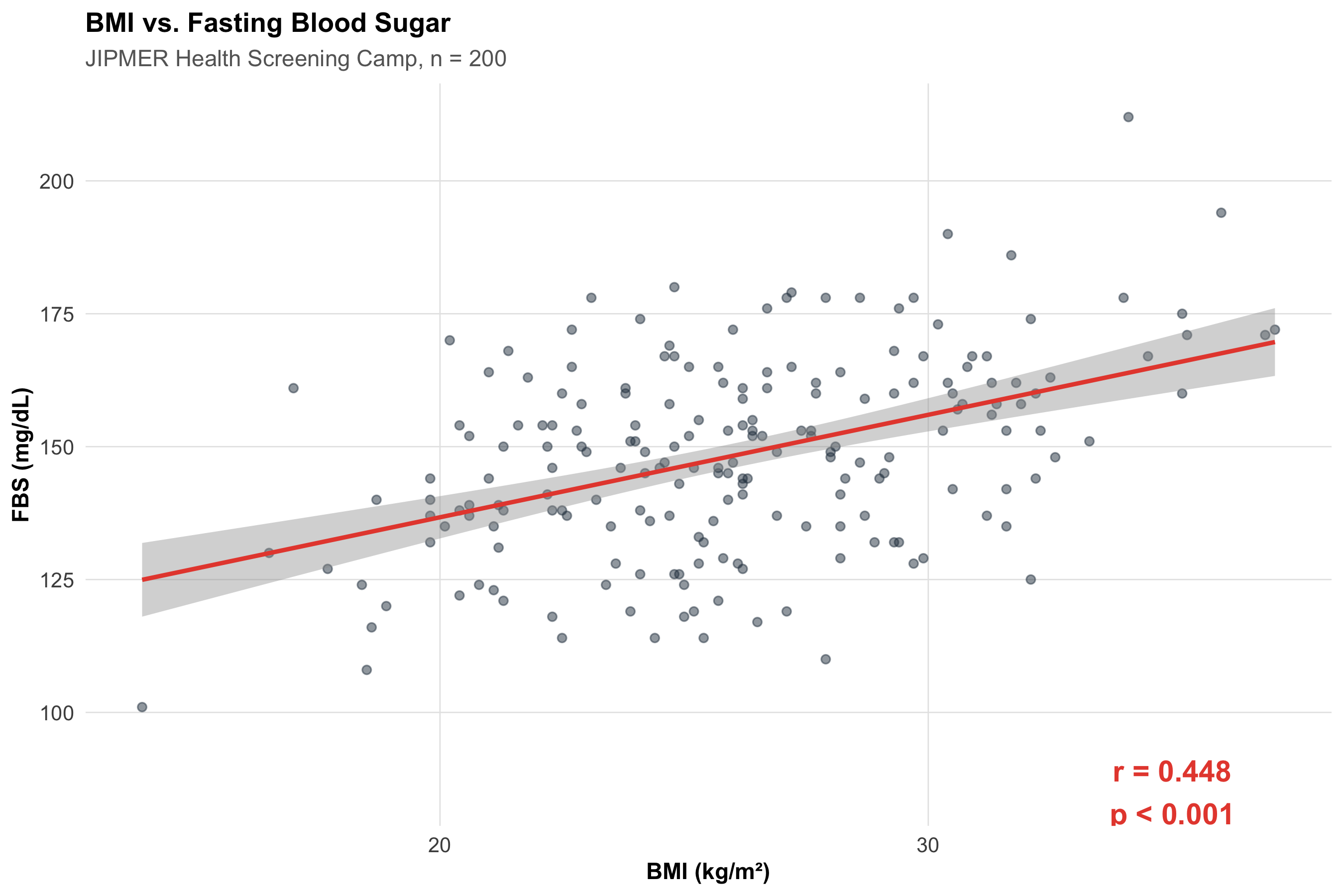
A research team at JIPMER, Puducherry, is studying whether higher BMI is associated with higher fasting blood sugar (FBS) in 200 adults attending a health screening camp. They plot the data and see what looks like a positive trend. But the questions cascade:

1. How strong is the association? (Correlation)
2. Can we predict FBS from BMI? (Simple linear regression)
3. Does the association persist after adjusting for age and sex? (Multiple regression)
4. If the outcome were diabetes (yes/no) rather than FBS, what model should they use? (Logistic regression)

This module builds each tool in sequence.

---

12.3 Section 1: Correlation

1.1 What Correlation Measures

Correlation quantifies the strength and direction of the linear relationship between two continuous variables.

In words: As one variable goes up, does the other tend to go up (positive), go down (negative), or show no pattern (zero)?

\[r = \frac{\sum (x_i - \bar{x})(y_i - \bar{y})}{\sqrt{\sum (x_i - \bar{x})^2 \cdot \sum (y_i - \bar{y})^2}}\]

Conceptually: r = average of the products of standardised deviations = Covariance(x, y) / (SD_x × SD_y).

Range: −1 (perfect negative) to +1 (perfect positive). r = 0 means no linear association.

---

1.2 Generating the Data

# 200 adults at JIPMER health camp
n <- 200
age <- round(rnorm(n, mean = 45, sd = 12))
bmi <- round(rnorm(n, mean = 26, sd = 4.5), 1)
# FBS partly driven by BMI + age + noise
fbs <- round(80 + 1.8 * bmi + 0.5 * age + rnorm(n, sd = 15))

health <- data.frame(
  ID = 1:n, Age = age, BMI = bmi, FBS = fbs,
  Sex = sample(c("Male", "Female"), n, replace = TRUE)
)

cat("First 6 rows:\n")

First 6 rows:

head(health)

  ID Age  BMI FBS    Sex
1  1  61 17.0 161 Female
2  2  38 27.5 135 Female
3  3  49 31.3 162 Female
4  4  53 35.3 171 Female
5  5  50 19.8 132 Female
6  6  44 20.8 124   Male

---

1.3 Pearson Correlation: Worked Example

r_bmi_fbs <- cor(health$BMI, health$FBS)
cor_test <- cor.test(health$BMI, health$FBS)

ggplot(health, aes(x = BMI, y = FBS)) +
  geom_point(alpha = 0.5, color = "#2c3e50") +
  geom_smooth(method = "lm", se = TRUE, color = "#e74c3c", linewidth = 1) +
  annotate("text", x = 35, y = 85,
           label = paste0("r = ", round(r_bmi_fbs, 3),
                         "\np < 0.001"),
           fontface = "bold", size = 5, color = "#e74c3c") +
  labs(title = "BMI vs. Fasting Blood Sugar",
       subtitle = "JIPMER Health Screening Camp, n = 200",
       x = "BMI (kg/m²)", y = "FBS (mg/dL)") +
  theme_clean()

Interpretation: r = 0.448 — a moderate positive correlation. As BMI increases, FBS tends to increase. The p-value tests H₀: ρ = 0 (no linear association in the population).

Interpreting Correlation Strength

	r
0.00 – 0.19	Negligible
0.20 – 0.39	Weak
0.40 – 0.59	Moderate
0.60 – 0.79	Strong
0.80 – 1.00	Very strong

These are rough guidelines — clinical context matters. A correlation of 0.3 between a biomarker and disease may be clinically important.

---

1.4 Spearman Rank Correlation

When the relationship is monotonic but not linear, or the data are ordinal, use Spearman’s rₛ (rank-based):

# Severity score (ordinal 1-5) vs. hospital LOS
severity <- sample(1:5, 60, replace = TRUE, prob = c(0.15, 0.25, 0.3, 0.2, 0.1))
los <- severity * 2 + rpois(60, lambda = 3) + round(rexp(60, rate = 0.3))

rs <- cor(severity, los, method = "spearman")
cat("Spearman rₛ =", round(rs, 3), "\n")

Spearman rₛ = 0.716 

Pearson vs. Spearman

Feature	Pearson (r)	Spearman (rₛ)
Relationship type	Linear	Monotonic (any shape)
Data type	Continuous, roughly normal	Ordinal or skewed continuous
Sensitive to outliers?	Yes — a single outlier can flip r	No — works on ranks
When to use	Both variables continuous, linear scatter	Ordinal data, skewed, or outliers present

---

1.5 Correlation ≠ Causation

The Ice-Cream-Drowning Fallacy

In summer months, ice cream sales and drowning deaths both rise. The correlation is strong (r ≈ 0.8). Should we ban ice cream?

No. The lurking variable is temperature — warm weather drives both.

Sources of spurious association include confounding (a third variable drives both), reverse causality (y causes x), selection bias (how the sample was chosen), and measurement error.

A strong r tells you the variables move together, not that one causes the other.

---

12.4 Section 2: Simple Linear Regression

2.1 The Model

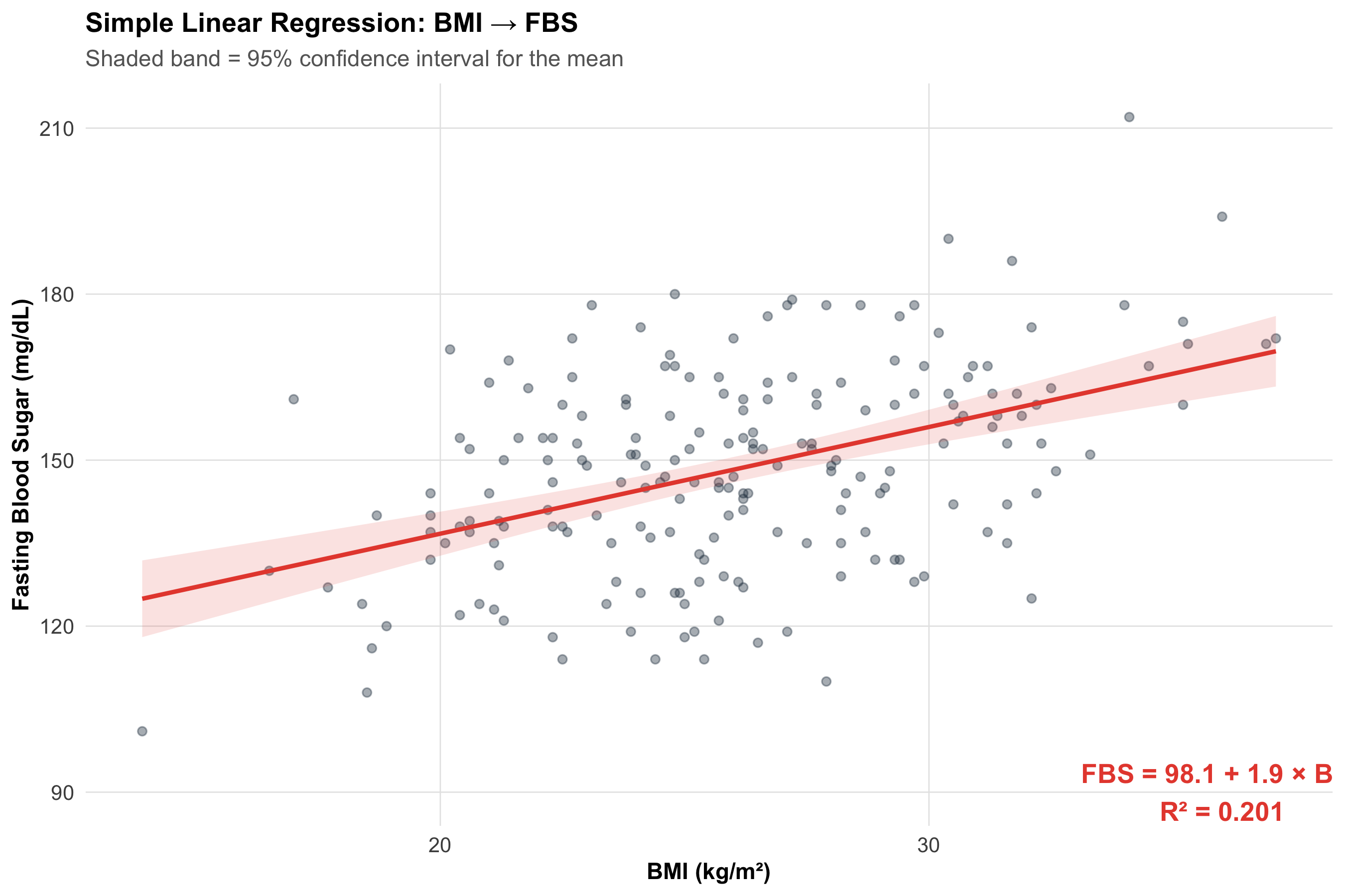
We want to predict FBS from BMI. Simple linear regression fits the equation:

In words: Predicted outcome = Baseline level + (Rate of change × Predictor) + Random error

\[y = \beta_0 + \beta_1 x + \varepsilon\]

where:

• \(\beta_0\) = intercept (predicted y when x = 0)
• \(\beta_1\) = slope (change in y for each 1-unit increase in x)
• \(\varepsilon\) = random error (what the model can’t explain)

The method of least squares finds \(\beta_0\) and \(\beta_1\) that minimise \(\sum (y_i - \hat{y}_i)^2\).

---

2.2 Fitting the Model in R

model <- lm(FBS ~ BMI, data = health)
summary(model)

Call:
lm(formula = FBS ~ BMI, data = health)

Residuals:
    Min      1Q  Median      3Q     Max 
-41.940 -11.390   0.357  10.531  48.106 

Coefficients:
            Estimate Std. Error t value Pr(>|t|)    
(Intercept)  98.1466     7.2100  13.613  < 2e-16 ***
BMI           1.9281     0.2732   7.058 2.78e-11 ***
---
Signif. codes:  0 '***' 0.001 '**' 0.01 '*' 0.05 '.' 0.1 ' ' 1

Residual standard error: 16.42 on 198 degrees of freedom
Multiple R-squared:  0.201, Adjusted R-squared:  0.197 
F-statistic: 49.81 on 1 and 198 DF,  p-value: 2.784e-11

coefs <- tidy(model, conf.int = TRUE)
b0 <- coefs$estimate[1]
b1 <- coefs$estimate[2]

cat("Regression equation:\n")

Regression equation:

cat("FBS =", round(b0, 2), "+", round(b1, 2), "× BMI\n")

FBS = 98.15 + 1.93 × BMI

cat("\nInterpretation:\n")

Interpretation:

cat("For each 1 kg/m² increase in BMI, FBS increases by",
    round(b1, 2), "mg/dL on average.\n")

For each 1 kg/m² increase in BMI, FBS increases by 1.93 mg/dL on average.

cat("95% CI for slope:", round(coefs$conf.low[2], 2),
    "to", round(coefs$conf.high[2], 2), "\n")

95% CI for slope: 1.39 to 2.47 

Interpreting the Slope

The slope \(\beta_1\) = 1.93 means: for every additional 1 kg/m² of BMI, fasting blood sugar increases by about 1.9 mg/dL, holding nothing else constant.

The intercept \(\beta_0\) = 98.1 is the predicted FBS when BMI = 0 — biologically meaningless here, but mathematically necessary to position the line.

---

2.3 Visualising the Regression

ggplot(health, aes(x = BMI, y = FBS)) +
  geom_point(alpha = 0.4, color = "#2c3e50") +
  geom_smooth(method = "lm", se = TRUE, color = "#e74c3c", fill = "#e74c3c",
              alpha = 0.15, linewidth = 1) +
  annotate("text", x = 36, y = 90,
           label = paste0("FBS = ", round(b0, 1), " + ",
                         round(b1, 1), " × BMI\nR² = ",
                         round(summary(model)$r.squared, 3)),
           fontface = "bold", color = "#e74c3c", size = 4.5) +
  labs(title = "Simple Linear Regression: BMI → FBS",
       subtitle = "Shaded band = 95% confidence interval for the mean",
       x = "BMI (kg/m²)", y = "Fasting Blood Sugar (mg/dL)") +
  theme_clean()

---

2.4 R²: How Much Variance Is Explained?

In words: R² tells you what fraction of the total scatter in y is “explained” by the regression line.

\[R^2 = 1 - \frac{\text{Residual SS}}{\text{Total SS}} = 1 - \frac{\sum(y_i - \hat{y}_i)^2}{\sum(y_i - \bar{y})^2}\]

For simple regression, \(R^2 = r^2\) (the square of the Pearson correlation).

r_sq <- summary(model)$r.squared
cat("R² =", round(r_sq, 4), "\n")

R² = 0.201 

cat("BMI explains", round(r_sq * 100, 1), "% of the variation in FBS.\n")

BMI explains 20.1 % of the variation in FBS.

cat("The remaining", round((1 - r_sq) * 100, 1),
    "% is due to age, diet, genetics, measurement error, etc.\n")

The remaining 79.9 % is due to age, diet, genetics, measurement error, etc.

What Is a ‘Good’ R²?

There is no universal threshold. In clinical prediction models, R² = 0.3–0.5 may be useful. In lab assays, R² > 0.95 is expected. Always ask: “Is this model useful for the clinical question?”

---

2.5 Confidence Interval vs. Prediction Interval

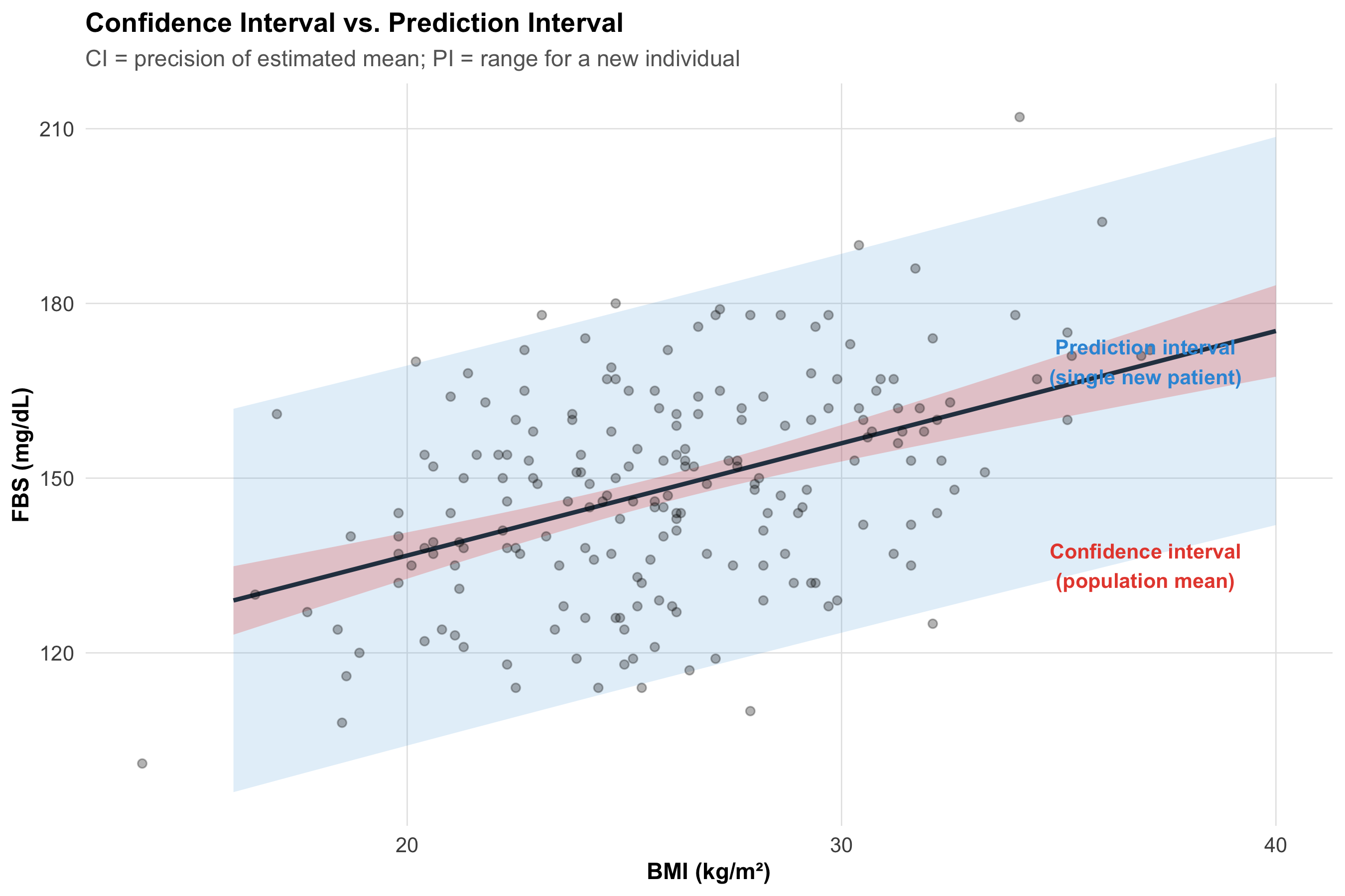
new_data <- data.frame(BMI = seq(16, 40, by = 0.5))
ci_pred <- predict(model, newdata = new_data, interval = "confidence")
pi_pred <- predict(model, newdata = new_data, interval = "prediction")

plot_data <- data.frame(
  BMI = new_data$BMI,
  Fit = ci_pred[, "fit"],
  CI_lower = ci_pred[, "lwr"], CI_upper = ci_pred[, "upr"],
  PI_lower = pi_pred[, "lwr"], PI_upper = pi_pred[, "upr"]
)

ggplot() +
  geom_ribbon(data = plot_data, aes(x = BMI, ymin = PI_lower, ymax = PI_upper),
              fill = "#3498db", alpha = 0.15) +
  geom_ribbon(data = plot_data, aes(x = BMI, ymin = CI_lower, ymax = CI_upper),
              fill = "#e74c3c", alpha = 0.25) +
  geom_line(data = plot_data, aes(x = BMI, y = Fit), color = "#2c3e50",
            linewidth = 1) +
  geom_point(data = health, aes(x = BMI, y = FBS), alpha = 0.3) +
  annotate("text", x = 37, y = 170, label = "Prediction interval\n(single new patient)",
           color = "#3498db", fontface = "bold", size = 3.5) +
  annotate("text", x = 37, y = 135, label = "Confidence interval\n(population mean)",
           color = "#e74c3c", fontface = "bold", size = 3.5) +
  labs(title = "Confidence Interval vs. Prediction Interval",
       subtitle = "CI = precision of estimated mean; PI = range for a new individual",
       x = "BMI (kg/m²)", y = "FBS (mg/dL)") +
  theme_clean()

CI vs. PI

• Confidence interval (narrow, red): Where we expect the average FBS to lie for all people with a given BMI. It reflects uncertainty in the regression line itself.
• Prediction interval (wide, blue): Where we expect a single new patient’s FBS to lie. It includes both line uncertainty and individual variation.

Clinical prediction models report PIs. Research papers typically report CIs.

---

12.5 Section 3: Regression Assumptions and Diagnostics

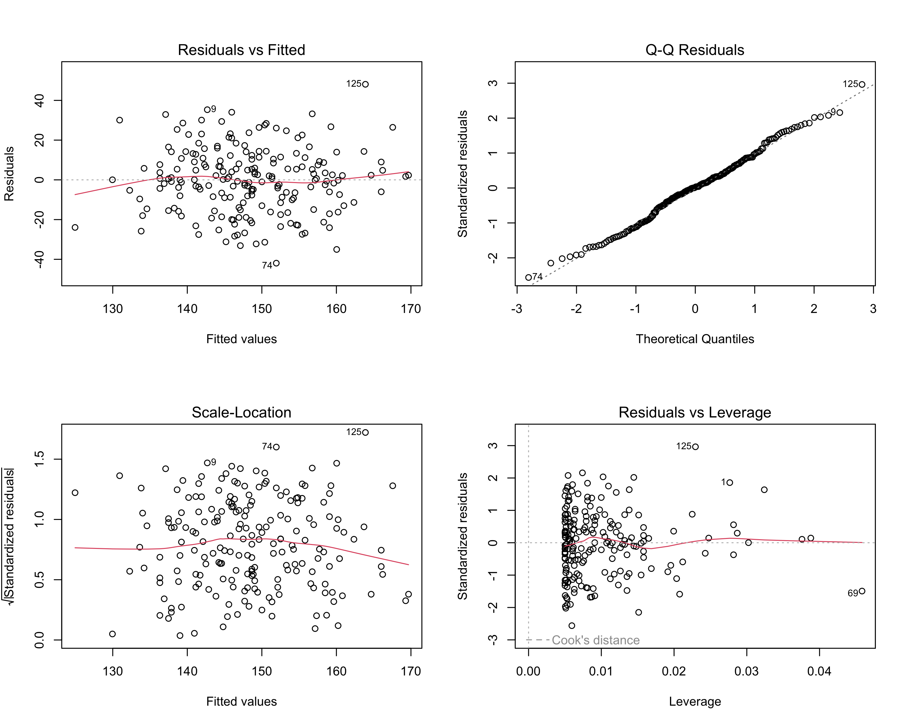
The four key assumptions (LINE):

1. Linearity — the relationship between x and y is linear
2. Independence — observations are independent
3. Normality — residuals are approximately normally distributed
4. Equal variance (homoscedasticity) — spread of residuals is constant across fitted values

3.1 Diagnostic Plots

par(mfrow = c(2, 2))
plot(model)

How to read these:

• Residuals vs. Fitted: Should be a random cloud. Patterns (curves, funnels) indicate non-linearity or heteroscedasticity.
• Q-Q plot: Points should follow the diagonal. Deviations at the tails suggest non-normal residuals.
• Scale-Location: Should show a roughly flat red line. An upward trend suggests increasing variance.
• Residuals vs. Leverage: Points in the upper/lower right (high leverage, large residual) may be influential — check Cook’s distance > 0.5.

---

3.2 What to Do When Assumptions Fail

Problem	Detection	Solution
Non-linear relationship	Curved pattern in residuals vs. fitted	Transform x or y (log, sqrt); add polynomial term
Non-normal residuals	Deviation from diagonal on Q-Q plot	Transform y; use robust regression; often OK if n > 30
Heteroscedasticity (funnel shape)	Spread increases with fitted values	Transform y (log); use weighted least squares; robust SE
Influential outliers	Cook's distance > 0.5 or 1	Investigate data entry errors; report results with and without

---

12.6 Section 4: Multiple Regression

4.1 Why Adjust for Confounders?

In our JIPMER data, BMI and FBS are associated — but age also influences FBS. Is the BMI–FBS association genuine, or is it partly (or entirely) confounded by age?

Multiple regression lets us ask: “What is the effect of BMI on FBS, holding age and sex constant?”

\[\text{FBS} = \beta_0 + \beta_1 \times \text{BMI} + \beta_2 \times \text{Age} + \beta_3 \times \text{Sex} + \varepsilon\]

In words: Each coefficient tells you the effect of that variable while all others are held fixed.

---

4.2 Fitting the Multiple Regression

model_multi <- lm(FBS ~ BMI + Age + Sex, data = health)
summary(model_multi)

Call:
lm(formula = FBS ~ BMI + Age + Sex, data = health)

Residuals:
    Min      1Q  Median      3Q     Max 
-39.198  -9.294  -0.238   9.588  46.001 

Coefficients:
            Estimate Std. Error t value Pr(>|t|)    
(Intercept)  74.9954     8.3993   8.929 3.12e-16 ***
BMI           2.0149     0.2605   7.734 5.35e-13 ***
Age           0.4315     0.0951   4.537 9.92e-06 ***
SexMale       3.3145     2.2089   1.501    0.135    
---
Signif. codes:  0 '***' 0.001 '**' 0.01 '*' 0.05 '.' 0.1 ' ' 1

Residual standard error: 15.61 on 196 degrees of freedom
Multiple R-squared:  0.2857,    Adjusted R-squared:  0.2747 
F-statistic: 26.13 on 3 and 196 DF,  p-value: 2.917e-14

coefs_simple <- tidy(model, conf.int = TRUE)
coefs_multi  <- tidy(model_multi, conf.int = TRUE)

comparison <- tibble(
  Variable = c("BMI (simple)", "BMI (adjusted)"),
  Estimate = c(coefs_simple$estimate[2], coefs_multi$estimate[2]),
  `95% CI` = c(
    paste0(round(coefs_simple$conf.low[2], 2), " to ", round(coefs_simple$conf.high[2], 2)),
    paste0(round(coefs_multi$conf.low[2], 2), " to ", round(coefs_multi$conf.high[2], 2))
  ),
  p = c(format(coefs_simple$p.value[2], digits = 3),
        format(coefs_multi$p.value[2], digits = 3))
)

kable(comparison, format = "html") %>%
  kable_styling(full_width = FALSE, bootstrap_options = c("bordered"))

Variable	Estimate	95% CI	p
BMI (simple)	1.928072	1.39 to 2.47	2.78e-11
BMI (adjusted)	2.014947	1.5 to 2.53	5.35e-13

Reading Multiple Regression Output

• The BMI coefficient in the adjusted model tells you the effect of BMI independent of age and sex.
• If the coefficient changes substantially after adjustment, confounding was present.
• Adjusted R² penalises for the number of predictors and is more honest than raw R² for comparing models.

---

4.3 Adjusted R² and Model Comparison

cat("Simple model R²:", round(summary(model)$r.squared, 4),
    "| Adj R²:", round(summary(model)$adj.r.squared, 4), "\n")

Simple model R²: 0.201 | Adj R²: 0.197 

cat("Multiple model R²:", round(summary(model_multi)$r.squared, 4),
    "| Adj R²:", round(summary(model_multi)$adj.r.squared, 4), "\n")

Multiple model R²: 0.2857 | Adj R²: 0.2747 

cat("\nAdding age and sex explains an additional",
    round((summary(model_multi)$r.squared - summary(model)$r.squared) * 100, 1),
    "% of FBS variance.\n")

Adding age and sex explains an additional 8.5 % of FBS variance.

Overfitting

Adding more predictors always increases R² — even if the new variables are noise. Adjusted R² corrects for this. If adjusted R² drops when you add a variable, that variable is not improving the model.

---

12.7 Section 5: Logistic Regression

5.1 When the Outcome Is Binary

What if the research question is: “Does higher BMI predict diabetes (yes/no)?”

FBS is continuous — but diabetes status is binary. Linear regression can’t model binary outcomes properly (it predicts values outside 0–1). We need logistic regression.

In words: Logistic regression models the log-odds of the outcome:

\[\ln\left(\frac{p}{1-p}\right) = \beta_0 + \beta_1 x\]

where \(p\) = probability of the event (diabetes = yes).

The odds ratio for a 1-unit increase in x is:

\[OR = e^{\beta_1}\]

---

5.2 Generating Binary Outcome Data

# Create diabetes outcome (higher BMI and age → higher probability)
health$diabetes_prob <- plogis(-8 + 0.15 * health$BMI + 0.05 * health$Age)
health$Diabetes <- rbinom(n, 1, health$diabetes_prob)
health$Diabetes_label <- ifelse(health$Diabetes == 1, "Diabetic", "Non-diabetic")

cat("Diabetes prevalence:", round(mean(health$Diabetes) * 100, 1), "%\n")

Diabetes prevalence: 13.5 %

---

5.3 Fitting the Logistic Regression

logit_model <- glm(Diabetes ~ BMI + Age + Sex, data = health, family = binomial)
summary(logit_model)

Call:
glm(formula = Diabetes ~ BMI + Age + Sex, family = binomial, 
    data = health)

Coefficients:
            Estimate Std. Error z value Pr(>|z|)    
(Intercept) -7.88632    1.78488  -4.418 9.94e-06 ***
BMI          0.15608    0.05142   3.035   0.0024 ** 
Age          0.04543    0.02000   2.271   0.0232 *  
SexMale     -0.66062    0.44725  -1.477   0.1397    
---
Signif. codes:  0 '***' 0.001 '**' 0.01 '*' 0.05 '.' 0.1 ' ' 1

(Dispersion parameter for binomial family taken to be 1)

    Null deviance: 158.31  on 199  degrees of freedom
Residual deviance: 141.55  on 196  degrees of freedom
AIC: 149.55

Number of Fisher Scoring iterations: 5

logit_coefs <- tidy(logit_model, conf.int = TRUE, exponentiate = TRUE)

or_table <- logit_coefs %>%
  filter(term != "(Intercept)") %>%
  select(Variable = term, OR = estimate, CI_low = conf.low, CI_high = conf.high,
         p = p.value) %>%
  mutate(across(c(OR, CI_low, CI_high), ~ round(., 3)),
         p = format(p, digits = 3))

kable(or_table, col.names = c("Variable", "OR", "95% CI Lower", "95% CI Upper", "p-value"),
      format = "html") %>%
  kable_styling(full_width = FALSE, bootstrap_options = c("bordered", "hover"))

Variable	OR	95% CI Lower	95% CI Upper	p-value
BMI	1.169	1.060	1.299	0.0024
Age	1.046	1.007	1.090	0.0232
SexMale	0.517	0.208	1.220	0.1397

Interpreting Logistic Regression ORs

• OR for BMI: For each 1 kg/m² increase in BMI, the odds of diabetes change by a factor of 1.17 (holding age and sex constant).
• OR > 1: Higher BMI increases the odds of diabetes.
• OR < 1: The variable is protective.
• 95% CI excluding 1.0: Statistically significant.

This connects directly to the Odds Ratio from Module 10 — logistic regression is the multivariable extension of the 2×2 table OR.

---

5.4 Predicted Probabilities

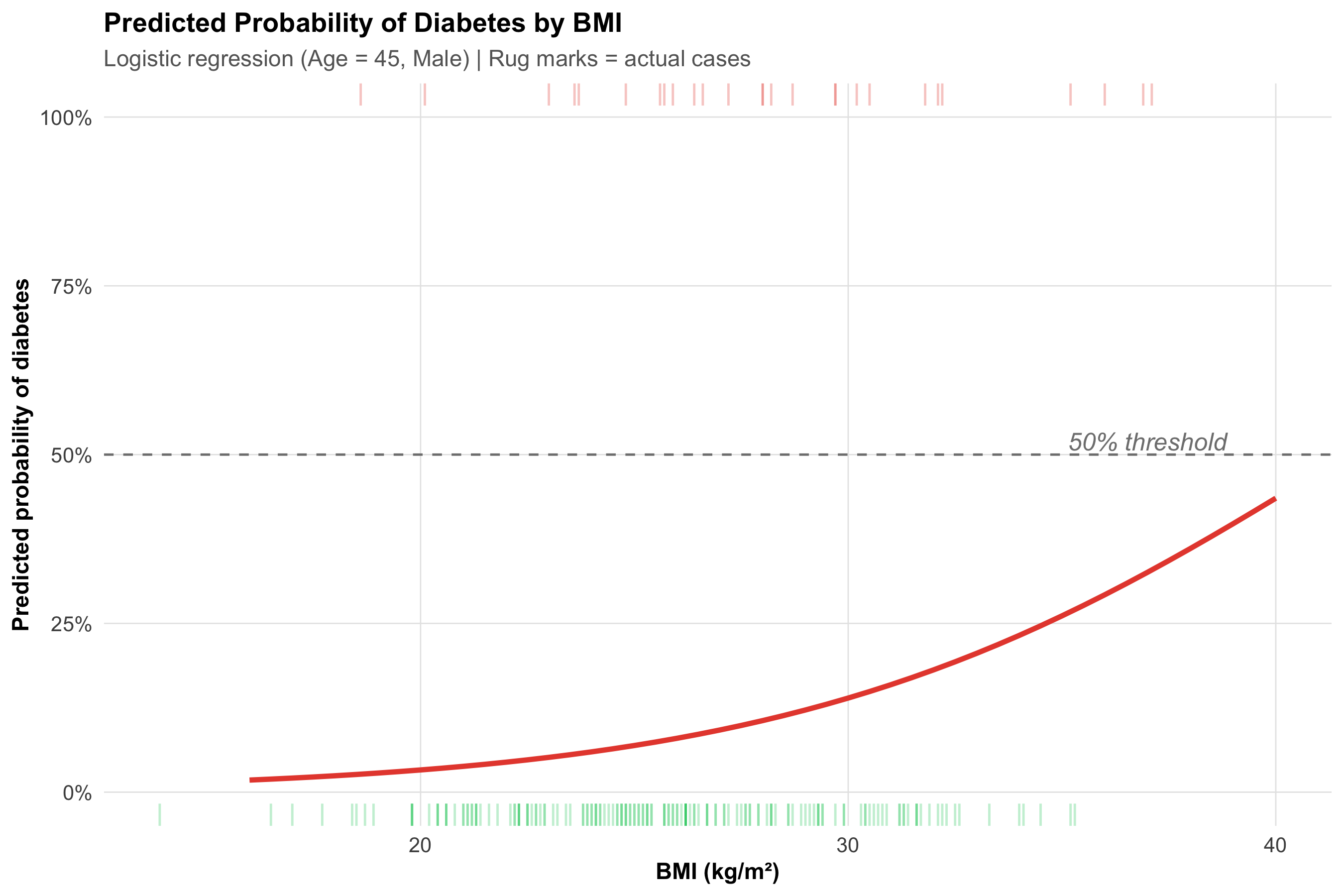
bmi_seq <- data.frame(BMI = seq(16, 40, by = 0.5), Age = 45, Sex = "Male")
bmi_seq$pred_prob <- predict(logit_model, newdata = bmi_seq, type = "response")

ggplot(bmi_seq, aes(x = BMI, y = pred_prob)) +
  geom_line(color = "#e74c3c", linewidth = 1.2) +
  geom_rug(data = health %>% filter(Diabetes == 1), aes(x = BMI, y = NULL),
           sides = "t", alpha = 0.3, color = "#e74c3c") +
  geom_rug(data = health %>% filter(Diabetes == 0), aes(x = BMI, y = NULL),
           sides = "b", alpha = 0.3, color = "#2ecc71") +
  geom_hline(yintercept = 0.5, linetype = "dashed", color = "gray50") +
  annotate("text", x = 37, y = 0.52, label = "50% threshold",
           color = "gray50", fontface = "italic") +
  scale_y_continuous(labels = percent_format(), limits = c(0, 1)) +
  labs(title = "Predicted Probability of Diabetes by BMI",
       subtitle = "Logistic regression (Age = 45, Male) | Rug marks = actual cases",
       x = "BMI (kg/m²)", y = "Predicted probability of diabetes") +
  theme_clean()

The S-shaped (sigmoid) curve is the hallmark of logistic regression. The probability is bounded between 0 and 1 — unlike linear regression, which would predict impossible values.

---

12.8 Section 6: The Correlation–Causation–Regression Framework

Correlation → Regression → Causation?

Tool	What it tells you	What it does NOT tell you
Correlation (r)	Strength and direction of linear association	Whether x causes y
Simple regression	How y changes per unit of x; prediction	Whether the relationship is causal
Multiple regression	Effect of x adjusted for confounders	Whether all confounders are measured
Logistic regression	OR for binary outcomes, adjusted	Causation without proper study design

Regression adjusts for measured confounders — but unmeasured confounders can still bias results. Only a well-designed RCT (Module 7) can establish causation. Regression in observational data provides adjusted associations, not proof of causation.

---

12.9 Section 7: Decision Framework

Scenario	Method	Output
Two continuous variables — strength of association?	Pearson correlation (r)	r, p-value, 95% CI
Ordinal data or outliers present?	Spearman rank correlation (rₛ)	rₛ, p-value
Predict continuous outcome from one predictor?	Simple linear regression	Slope, R², equation, CI/PI
Predict continuous outcome, adjust for confounders?	Multiple linear regression	Adjusted slopes, adjusted R²
Predict binary outcome (yes/no)?	Logistic regression	Odds ratios, predicted probabilities
Predict time-to-event (survival)?	Cox regression (Module 12)	Hazard ratios

---

12.10 Summary

Key Takeaways

1. Pearson r measures linear association (−1 to +1). Spearman rₛ is the rank-based alternative for ordinal or skewed data.

2. Correlation ≠ causation. Confounding, reverse causality, and selection bias can create spurious associations.

3. Simple linear regression fits y = β₀ + β₁x. The slope is the change in y per 1-unit increase in x. R² = fraction of variance explained.

4. Always check LINE assumptions — linearity, independence, normality of residuals, equal variance. Use diagnostic plots.

5. Confidence intervals (for the mean) are narrower than prediction intervals (for a new individual). Always report uncertainty.

6. Multiple regression adjusts for confounders: “effect of x₁ holding x₂, x₃, … constant.” Use adjusted R² for model comparison.

7. Logistic regression models binary outcomes. Coefficients exponentiate to odds ratios — connecting directly to Module 10.

8. No regression model proves causation in observational data. Regression adjusts for measured confounders; RCTs are needed for causal claims.

---

12.11 Practice Questions

Q1: Correlation vs Causation

A study finds r = 0.85 between hours of TV watched per day and BMI in 500 adults. Which interpretation is MOST appropriate?

A. Watching more TV causes weight gain B. There is a strong positive linear association between TV hours and BMI C. 85% of the variation in BMI is explained by TV watching D. The relationship is statistically significant but clinically irrelevant

✘ A. Watching more TV causes weight gain — Incorrect. Correlation does not establish causation — confounders like sedentary lifestyle, diet, and socioeconomic status may explain the association.

✔ B. There is a strong positive linear association between TV hours and BMI — Correct! r = 0.85 indicates a strong positive linear association. We cannot infer causation from correlation alone.

✘ C. 85% of the variation in BMI is explained by TV watching — Incorrect. R² (not r) gives the proportion of variance explained. R² = 0.85² = 0.72, meaning 72% — but this still doesn’t prove causation.

✘ D. The relationship is statistically significant but clinically irrelevant — Incorrect. r = 0.85 is both statistically and practically strong. Clinical relevance cannot be dismissed without context.

---

Q2: Regression Prediction

A regression model gives: SBP = 90 + 0.6 × Age (years). For a 60-year-old patient, what is the predicted systolic BP?

A. 90 mmHg B. 126 mmHg C. 150 mmHg D. 36 mmHg

✘ A. 90 mmHg — Incorrect. That is the intercept only — you need to add the age contribution: 0.6 × 60 = 36.

✔ B. 126 mmHg — Correct! SBP = 90 + 0.6 × 60 = 90 + 36 = 126 mmHg.

✘ C. 150 mmHg — Incorrect. Check the arithmetic: 90 + (0.6 × 60) = 126, not 150.

✘ D. 36 mmHg — Incorrect. 36 is the age contribution (0.6 × 60), but you must add the intercept (90).

---

Q3: R-Squared Interpretation

In a simple linear regression, R² = 0.64. Which statement is correct?

A. The correlation coefficient r = 0.64 B. The predictor explains 64% of the variation in the outcome C. The model correctly classifies 64% of observations D. The slope of the regression line is 0.64

✘ A. The correlation coefficient r = 0.64 — Incorrect. R² = r², so r = √0.64 = 0.80 (assuming positive association).

✔ B. The predictor explains 64% of the variation in the outcome — Correct! R² = 0.64 means 64% of outcome variance is explained by the model. The remaining 36% is unexplained.

✘ C. The model correctly classifies 64% of observations — Incorrect. R² is not a classification metric — it measures proportion of variance explained.

✘ D. The slope of the regression line is 0.64 — Incorrect. R² and the slope are different quantities. The slope depends on the units of x and y.

---

Q4: Logistic Regression OR

A logistic regression for diabetes (yes/no) gives OR = 1.12 (95% CI: 1.04–1.21) for BMI. What is the correct interpretation?

A. For each 1 kg/m² increase in BMI, the probability of diabetes increases by 12% B. For each 1 kg/m² increase in BMI, the odds of diabetes increase by 12%, and this is statistically significant C. BMI causes diabetes with 12% certainty D. The model explains 12% of the variance in diabetes

✘ A. For each 1 kg/m² increase in BMI, the probability of diabetes increases by 12% — Incorrect. OR is not the same as probability increase. The OR says the odds multiply by 1.12 per unit BMI increase.

✔ B. For each 1 kg/m² increase in BMI, the odds of diabetes increase by 12%, and this is statistically significant — Correct! OR = 1.12 means the odds multiply by 1.12 per unit BMI increase (12% increase). The CI excludes 1.0, so p < 0.05.

✘ C. BMI causes diabetes with 12% certainty — Incorrect. An OR does not express certainty of causation. It quantifies the association between BMI and odds of diabetes.

✘ D. The model explains 12% of the variance in diabetes — Incorrect. OR is not R². The 1.12 refers to the odds ratio per unit change in the predictor.

---

Q5: Regression Assumptions

Which of the following is NOT an assumption of simple linear regression?

A. Linearity of the relationship between x and y B. Independence of observations C. The predictor variable x must be normally distributed D. Homoscedasticity (constant variance of residuals)

✘ A. Linearity of the relationship between x and y — Incorrect — this IS a required assumption (the L in LINE).

✘ B. Independence of observations — Incorrect — this IS a required assumption (the I in LINE).

✔ C. The predictor variable x must be normally distributed — Correct! Regression assumes normality of residuals, not of x. The predictor can have any distribution.

✘ D. Homoscedasticity (constant variance of residuals) — Incorrect — this IS a required assumption (the E in LINE).

---

Q6: Confounding in Multiple Regression

A multiple regression shows that the association between BMI and FBS drops from β = 2.1 (simple) to β = 1.4 (after adjusting for age and sex). What does this suggest?

A. The original association was entirely spurious B. Age and sex are mediators in the causal pathway C. Age and/or sex were confounders — they partly explained the BMI–FBS association D. The multiple regression model is invalid

✘ A. The original association was entirely spurious — Incorrect. The adjusted coefficient is still 1.4 and presumably still significant — the association remains, just weaker.

✘ B. Age and sex are mediators in the causal pathway — Incorrect. Without a causal diagram, we cannot distinguish confounding from mediation based on coefficient change alone.

✔ C. Age and/or sex were confounders — they partly explained the BMI–FBS association — Correct! The coefficient dropped by ~33% after adjustment, suggesting age/sex confounded part (but not all) of the association.

✘ D. The multiple regression model is invalid — Incorrect. A coefficient change after adjustment is expected and informative — it means confounding was present and has been partially addressed.

---

12.12 Appendix: R Functions Quick Reference

# ======================================
# QUICK R REFERENCE — CORRELATION & REGRESSION
# ======================================

# Pearson correlation
cor(x, y)
cor.test(x, y)  # with p-value and 95% CI

# Spearman correlation
cor(x, y, method = "spearman")

# Simple linear regression
model <- lm(y ~ x, data = df)
summary(model)                       # coefficients, R², p-values
confint(model)                       # 95% CI for coefficients
predict(model, newdata, interval = "confidence")  # CI for mean
predict(model, newdata, interval = "prediction")  # PI for individual

# Diagnostic plots
par(mfrow = c(2,2)); plot(model)

# Multiple regression
model_multi <- lm(y ~ x1 + x2 + x3, data = df)
summary(model_multi)

# Logistic regression
logit <- glm(y ~ x1 + x2, data = df, family = binomial)
summary(logit)
exp(coef(logit))          # odds ratios
exp(confint(logit))       # 95% CI for ORs
predict(logit, type = "response")  # predicted probabilities

# Compare models
anova(model_simple, model_multi)
AIC(model_simple, model_multi)

---

End of Module 11

AIIMS Bhopal Biostatistics Course | Updated: 2026-02-25