---
title: "An Orientation to R"
subtitle: "Getting comfortable with R and RStudio"
author: "Dr Ashwini Kalantri"
format:
html:
toc: true
code-fold: show
code-tools: true
execute:
warning: false
message: false
---
## What This Session Is (and Isn't) {.unnumbered}
::: {.callout-warning}
This session is **not** an R programming course. You do not need to memorise anything here.
:::
The goal is to build enough familiarity that when you see R code in the following sessions, you can:
- Recognise what it is doing
- Know where to change an input value
- Run it yourself and see the output
- Not be intimidated by it
Think of this as learning to read a new language well enough to follow a conversation — not to write poetry.
## The RStudio Interface
When you open RStudio, you see four panels. Understanding what each one does will help you follow along in every session.
- **Source Editor (top-left):** Where you write and edit code files (`.R`, `.qmd`)
- **Console (bottom-left):** Where code runs and output appears
- **Environment (top-right):** Shows all variables and data currently in memory
- **Files / Plots / Help (bottom-right):** File browser, plot viewer, package documentation
For this workshop, you will mostly open a `.qmd` file in the Source panel, run code chunks by clicking the green ▶ button, and see results in the Console or Plots tab.
::: {.callout-important}
## Always open the project file first
Always open the workshop by double-clicking the `.Rproj` file in the workshop folder — not by opening `.qmd` files directly. This ensures R looks for files in the right place. If you skip this step, data import commands will fail with a `cannot open file` error.
:::
## The Workflow
Every session in this workshop follows the same four steps. Come back to this whenever you feel unsure about what to do next.
```{mermaid}
flowchart LR
  A["<b>READ</b><br/>the code<br/><i>(understand logic)</i>"]:::blue --> B["<b>MODIFY</b><br/>a parameter<br/><i>(change a number)</i>"]:::green --> C["<b>RUN</b><br/>the chunk<br/><i>(click play)</i>"]:::orange --> D["<b>INTERPRET</b><br/>the output<br/><i>(what changed?)</i>"]:::red
  D -. "Try again" .-> B

classDef blue   fill:#4e79a7,color:#fff
classDef green  fill:#59a14f,color:#fff
classDef orange fill:#f28e2b,color:#fff
classDef red    fill:#e15759,color:#fff
```
## Working with .qmd Files
All workshop materials are in **Quarto (.qmd)** files. These combine three things in one document:
- **Text** — plain-language explanations, like this paragraph
- **Code chunks** — grey blocks containing R code, with a green ▶ button to run them
- **Outputs** — results, tables, and plots that appear directly below each chunk
To work with a `.qmd` file, open it in RStudio, read the text explanations, and run code chunks one at a time using the ▶ button. Modify a value and re-run to see what changes. You can also click **Render** in the toolbar to produce a complete HTML document with everything formatted together.
## Your First Code
Run the chunk below to confirm everything is working. Click the green ▶ button.
```{r}
#| label: first-code
#| echo: true
print("Coding for better health decisions.")
```
If you see the text printed below the chunk, your setup is working correctly.
### Comments
In R, the `#` symbol marks a **comment** — anything after it on that line is ignored by R. Comments are notes for the human reading the code, not instructions for the computer. You will see them throughout every session. Read them — they are often the clearest explanation of what a section of code is doing.
```{r}
#| echo: true
#| eval: false
# Print the text
print("Coding for better health decisions.")

print("Coding for better health decisions.") # Print the text

# Multi-line comment
# about printing the text
print("Coding for better health decisions.")
```
## Assignment
In R, you store a value under a name using the **assignment operator** `<-`. Once stored, you can use the name anywhere in place of the value.
```{r}
#| label: assignment
#| echo: true
text <- "Coding for better health decisions."
print(text)
```
When you see `<-` in workshop code, you know: **this is where a value is stored, and this is what you change** to explore a different scenario.
You may occasionally see `->` or `=` used for assignment in older code. Prefer `<-` in your own work.
## Operators
### Arithmetic
R handles all standard arithmetic. These operators appear throughout model calculations for costs, probabilities, and outcomes.
```{r}
#| label: arithmetic
#| echo: true
2 + 5 # Addition
73 - 32 # Subtraction
47 * 7 # Multiplication
86 / 3 # Division
8 ^ 2 # Exponentiation
```
### Relational
Relational operators compare two values and return `TRUE` or `FALSE`. You will encounter these inside conditional checks — for example, testing whether an ICER is below a cost-effectiveness threshold.
```{r}
#| label: relational
#| echo: true
5 > 6 # Greater than
5 < 6 # Less than
6 == 6 # Equal to — note the double == for comparison, not single =
8 >= 5 # Greater than or equal to
7 <= 10 # Less than or equal to
9 != 10 # Not equal to
```
## Objects
In R, everything is stored as an **object**. The three types you will encounter most in this workshop are vectors, matrices, and data frames.
### Vectors
A vector is an ordered collection of values. Create one with `c()` — short for "combine".
```{r}
#| label: vectors
#| echo: true
vec <- c(2, 4, 6, 8, 3, 5.5)
vec
```
Vectors can also have **named elements** — a pattern you will see constantly in HTA models, where each value corresponds to a health state or treatment strategy:
```{r}
#| label: named-vectors
#| echo: true
costs <- c(treatment_A = 5000, treatment_B = 3000, treatment_C = 7000)
costs
```
You can retrieve a specific element by its position in the vector:
```{r}
#| echo: true
vec[5] # Fifth element of vec
```
### Matrix
A matrix is a two-dimensional object with rows and columns. In HTA, you will encounter matrices as **transition probability tables** for Markov models, where each cell holds the probability of moving from one health state to another.
```{r}
#| label: matrix
#| echo: true
mat <- matrix(1:36, nrow = 6, ncol = 6, byrow = FALSE)
mat
```
You can access a specific element, an entire column, or an entire row:
```{r}
#| echo: true
mat[3, 5] # Element at row 3, column 5
mat[, 5] # Entire column 5
mat[5, ] # Entire row 5
```
### Matrix multiplication
```{r}
#| label: matrix-mult
#| echo: true
mat1 <- matrix(c(3, 5, 1, 9), nrow = 2, ncol = 2, byrow = FALSE)
mat2 <- matrix(c(7, 4, 2, 8), nrow = 2, ncol = 2, byrow = FALSE)

mat1 %*% mat2
```
### Data Frames
A data frame is R's equivalent of a spreadsheet table — rows are observations, columns are variables.
```{r}
#| label: dataframe
#| echo: true
age    <- c(12, 24, NA, 23, 65, 33)          # NA = missing value

gender <- c("M", "F", "F", "M", "M", "F")

occu   <- factor(c(1, 4, 3, 2, 4, 5),        # factor() = categorical variable
                 levels = c(1:5),
                 labels = c("Unemp", "Service", "Student", "Business", "Prof"))

dob    <- c(as.Date("1993-01-16"),            # as.Date() converts text to a date
            as.Date("1963-12-24"),
            as.Date("1971-01-05"),
            as.Date("1982-11-11"),
            as.Date("1984-05-15"),
            as.Date("1999-03-07"))

df <- data.frame(age, gender, occu, dob)
df
```
You access a specific column using `$`:
```{r}
#| echo: true
df$age
```
## Functions
A function takes one or more inputs (called **arguments**), does something with them, and returns an output. The general syntax is:
```{r}
#| echo: true
#| eval: false
function_name(argument1 = value1, argument2 = value2, ...)
```
For example, `mean()` calculates the average of a vector. The `na.rm = TRUE` argument tells it to remove missing values before calculating — without it, a single `NA` in the data will make the result `NA`.
```{r}
#| echo: true
mean(x = df$age, na.rm = TRUE)
```
::: {.callout-tip}
## Getting help
Type `?` followed by any function name in the Console to open its documentation — arguments, return values, and worked examples:
```r
?mean
?round
?ggplot
```
:::
## Packages
R's base installation covers the basics. **Packages** are collections of additional functions written by the R community that extend what R can do. Install a package once, load it at the start of each session.
```{r}
#| label: packages
#| echo: true
#| eval: false
# Install a package — only need to do this once
install.packages("dplyr")
```
```{r}
#| echo: true
# Load a package — need to do this each session
library(dplyr)

dplyr::glimpse(df)
```
**Analogy:** Installing is like downloading an app. Loading is like opening it. In this workshop, the packages you need are listed at the top of each session file — you do not need to find or choose them yourself.
Key packages used in this workshop:
| Package | Purpose |
|---|---|
| `ggplot2` | Graphs and visualisation |
| `dplyr` | Data manipulation |
| `readxl`, `haven`, `rio` | Importing data |
| `heemod` | Markov cohort models |
| `BCEA`, `dampack` | Cost-effectiveness analysis |
| `flexsurv` | Survival modelling |
| `shiny` | Interactive web applications |
## Pipes
A pipe passes the output of one function directly into the next, letting you chain steps in a readable left-to-right sequence without creating intermediate objects. R has two pipe operators — `|>` (built into R) and `%>%` (from the `tidyverse`). They behave the same way in most situations.
```{r}
#| label: pipes
#| echo: true
df |>
  select(age, dob, occu) |>
  summarise(mean_age = mean(age, na.rm = TRUE))
```
Read this as: *take `df`, then select the age, dob, and occu columns, then calculate the mean age.* `select()` picks columns, `summarise()` calculates summaries. The pipe replaces deeply nested function calls with a sequence that reads the way you think.
## Importing Data
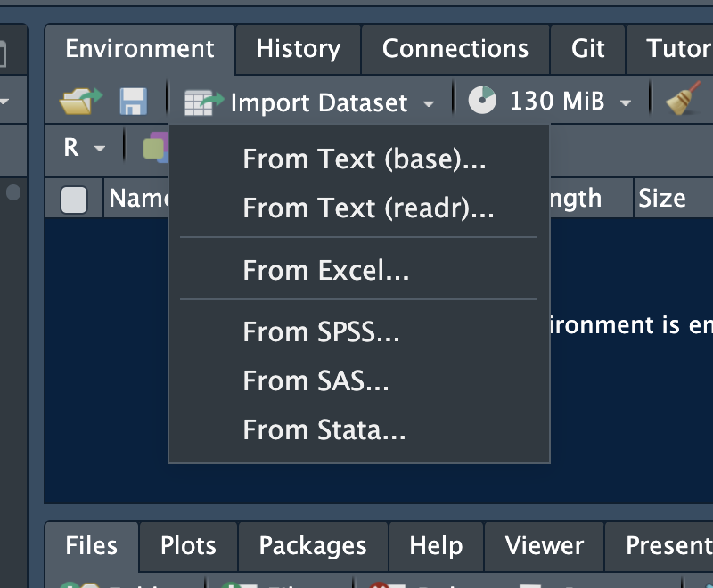
### Using the GUI
RStudio has a point-and-click import tool. Go to **File → Import Dataset** and choose your file type. RStudio generates the import code for you — a useful way to learn the syntax before writing it yourself.
### Importing with code
Once you know the syntax, code-based import is faster and fully reproducible:
```{r}
#| echo: true
#| eval: false
# CSV
data <- read.csv("files/data.csv")

# Excel
library(readxl)
data <- read_excel("files/data.xlsx")

# Stata and SPSS
library(haven)
data <- read_sav("files/data.sav")
data <- read_dta("files/data.dta")
```
The `rio` package provides a single `import()` function that detects the file format automatically — the simplest approach when you work with multiple file types:
```{r}
#| echo: true
#| eval: false
library(rio)
data <- rio::import("files/data.xlsx")
data <- rio::import("files/data.csv")
data <- rio::import("files/data.sav")
data <- rio::import("files/data.dta")
```
::: {.callout-important}
All import commands use **relative file paths** that only work when the `.Rproj` file has been opened first. A `cannot open file` error almost always means this step was skipped.
:::
## Loops
A `for` loop repeats a block of code a fixed number of times — once for each value in a sequence. In HTA modelling, loops are used to run the model across time cycles and across thousands of PSA iterations.
```{r}
#| label: loops
#| echo: true
library(rio)
data <- rio::import("files/data.csv")
library(dplyr)
data <- data |> mutate(bmi = round(wt / ((ht / 100)^2), 1))

for (i in 1:nrow(data)) {
  bmi <- round(data$wt[i] / ((data$ht[i] / 100)^2), 2)
  cat("BMI of Record No", i, "is", bmi, "\n")
}
```
When you see a `for` loop in the workshop code, you know: **the model is repeating a calculation**. You do not need to understand every line — just recognise that something is being done repeatedly, and that the values at the top of the loop control what is being repeated and how many times.
## Conditional Logic
An `if/else` block runs different code depending on whether a condition is `TRUE` or `FALSE`. You will see this used in cost-effectiveness decisions — is the ICER below the willingness-to-pay threshold? — and in model checks.
```{r}
#| echo: true
#| eval: false
if (condition) {
  # code to run if condition is TRUE
} else {
  # code to run if condition is FALSE
}
```
A simple example:
```{r}
#| label: conditional
#| echo: true
value <- 5000

if (value > 200) {
  cat("High")
} else {
  cat("Low")
}
```
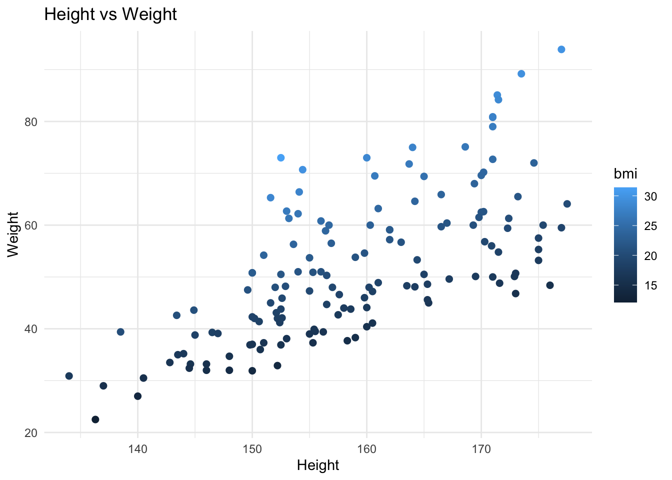
## Graphs
`ggplot2` is the standard package for data visualisation in R. It builds plots in layers — you start with the data, map variables to axes, then add geometric elements. The plot below uses the dataset imported in the Loops section.
```{r}
#| label: ggplot
#| echo: true
#| fig-cap: "Height vs Weight coloured by BMI"
library(ggplot2)

ggplot(data, aes(x = ht, y = wt, colour = bmi)) +
  geom_point(size = 2) +
  labs(x = "Height", y = "Weight", title = "Height vs Weight") +
  theme_minimal()
```
When you see `ggplot` in the workshop code, you know: **a chart is being created.** The `aes()` part maps variables to visual properties, the `geom_` function determines the chart type, and `labs()` sets the labels. Changing the data or the variables inside `aes()` changes the plot.
## Three Things to Remember
Almost nothing from this session needs to be memorised. Instead, keep these three things in mind throughout the workshop:
::: {.callout-note icon=false}
## 1. Values are stored with `<-`
Change them by editing the number on the right. Every exercise in this workshop is essentially this action.
:::
::: {.callout-note icon=false}
## 2. Code runs top to bottom
Run chunks in order. If you see an error about an object not being found, scroll up and run the chunks above first.
:::
::: {.callout-note icon=false}
## 3. Read the error message
It usually tells you exactly what went wrong — a missing package, a typo in a variable name, a file not found. Read it before asking for help.
:::
Everything else you can look up as needed — or ask an AI tool, as we will discuss in Session 7.
## Try It Yourself
Before moving to Session 3, modify the values below and re-run the chunk. Change the costs and QALYs to see how the ICER and the cost-effectiveness decision change.
```{r}
#| label: try-it
#| echo: true
# YOUR TASK: Change these values and re-run
cost_A <- 3000   # Cost of intervention A in ₹
cost_B <- 1500   # Cost of intervention B in ₹
qaly_A <- 0.82   # QALYs gained with A
qaly_B <- 0.75   # QALYs gained with B

# ── Do not modify below this line ─────────────────────────────────────────────

icer <- (cost_A - cost_B) / (qaly_A - qaly_B)
cat("ICER = ₹", round(icer, 0), "per QALY gained\n")
wtp <- 100000
if (icer < wtp) {
  cat("→ Cost-effective at WTP = ₹", format(wtp, big.mark = ",", scientific = FALSE), "\n")
} else {
  cat("→ NOT cost-effective at WTP = ₹", format(wtp, big.mark = ",", scientific = FALSE), "\n")
}
```
If you ran this and changed the result — you are ready for the rest of the workshop.
---
## Quick Reference {.unnumbered}
| Concept | Syntax | Example |
|---|---|---|
| Assign a value | `name <- value` | `cost <- 5000` |
| Named vector | `c(name = value)` | `c(A = 5000, B = 3000)` |
| Index a vector | `vec[n]` | `vec[5]` |
| Matrix multiply | `%*%` | `trace %*% tm` |
| Access a column | `df$col` | `df$age` |
| Function syntax | `fn(arg = val)` | `mean(x, na.rm = TRUE)` |
| Pipe | `\|>` | `df \|> select(age)` |
| If / else | `if (cond) {} else {}` | `if (icer < wtp) {...}` |
| Get help | `?function` | `?mean` |
| Comment | `#` | `# this is a note` |
---
*Session 2 · R for HTA (Basics) · RRC-HTA, AIIMS Bhopal*


Comments
In R, the
#symbol marks a comment — anything after it on that line is ignored by R. Comments are notes for the human reading the code, not instructions for the computer. You will see them throughout every session. Read them — they are often the clearest explanation of what a section of code is doing.Code