Session 4: Therapeutic Decision Tree — DES vs BMS
Drug-eluting stents vs bare metal stents for coronary artery disease in India
1. The Clinical Question
Coronary artery disease (CAD) is a leading cause of mortality in India. Percutaneous coronary intervention (PCI) with stent placement is a standard treatment, and the choice between drug-eluting stents (DES) and bare metal stents (BMS) has major cost and outcome implications.
In 2017, India’s NPPA capped stent prices — BMS at approximately ₹7,260 and DES at ₹29,600. As of 2025, revised ceilings stand at approximately ₹10,693 for BMS and ₹38,933 for DES. This dramatically changed the economics of stent choice in India.
The HTA question: At current Indian price ceilings, is DES cost-effective compared to BMS over a 5-year time horizon?
This is a therapeutic decision tree — comparing two treatment strategies with different costs and probabilities of downstream events.
2. Framing the Decision Problem — PICO
Before we touch any data, let us formalise the question using the PICO framework, extended for HTA.
TipWhy PICO matters for modelling
Every HTA model answers a specific question. The PICO forces us to be precise: which patients? which interventions? what are we measuring? The HTA extensions add the economic lens — whose costs count (perspective), how far we look (time horizon), how we value future outcomes (discounting), and when we say “worth it” (WTP threshold).
Notice that changing any element of the PICO changes the entire model. Younger patients? Different probabilities. Different country? Different costs and thresholds. This is why we build models in code — so we can adapt them.
3. Conceptual Map — What Do We Need?
Now that we know what we’re asking, let’s brainstorm: what information do we need to answer it?
Before looking up a single number, think about the building blocks of a cost-effectiveness model.
Code
mindmap
  root((DES vs BMS<br/>What do we need?))
    **Cohort**
      Who are we modelling?
      How many patients?
      How long do we follow them?
    **Probabilities**
      Does the procedure succeed?
      Does restenosis occur?
      Does a major event happen?
      What kind — MI or death?
    **Costs ₹**
      Stent itself
      PCI procedure
      Medications post-PCI
      Follow-up visits
      Repeat intervention if restenosis
      Managing MI or death
    **Utilities QALYs**
      Quality of life when well
      Quality after restenosis recovery
      Quality after surviving MI
      Death = 0
    **Framework**
      Time horizon
      Discount rate
      WTP threshold
      Perspective
mindmap
root((DES vs BMS<br/>What do we need?))
**Cohort**
Who are we modelling?
How many patients?
How long do we follow them?
**Probabilities**
Does the procedure succeed?
Does restenosis occur?
Does a major event happen?
What kind — MI or death?
**Costs ₹**
Stent itself
PCI procedure
Medications post-PCI
Follow-up visits
Repeat intervention if restenosis
Managing MI or death
**Utilities QALYs**
Quality of life when well
Quality after restenosis recovery
Quality after surviving MI
Death = 0
**Framework**
Time horizon
Discount rate
WTP threshold
Perspective
NoteThink before you code
This is how HTA analysts work in practice. You sketch the model on a whiteboard first, identify what data you need, then go find the numbers. The mind map above is your shopping list — now let’s fill in each category.
4. Input Parameters — One Category at a Time
4a. The Cohort
Every model starts with: who are we modelling, for how long, and what economic rules apply?
Code
# === COHORT & FRAMEWORK ===
n_cohort      <- 1000   # 1,000 patients undergoing PCI
time_horizon  <- 5      # years of follow-up
discount_rate <- 0.03   # 3% annual discount (years 2–5)
4b. Probabilities — What Can Happen?
These are the clinical evidence inputs. Each number comes from trials, registries, or meta-analyses.
Code
# === PROBABILITIES ===

# Procedural success
# Source: Indian PCI registry data
p_success_des <- 0.97
p_success_bms <- 0.96

# Restenosis within 1 year (requiring repeat revascularisation)
# Source: PMC comparative study (Indian data); international meta-analyses
p_restenosis_des <- 0.08   # DES: 5–10%
p_restenosis_bms <- 0.20   # BMS: 15–20%

# MACE at 5 years (MI or cardiac death)
# Among patients WITHOUT restenosis
p_mace_des_no_restenosis <- 0.08
p_mace_bms_no_restenosis <- 0.15

# Among patients WITH restenosis (after repeat revascularisation)
p_mace_des_restenosis <- 0.15
p_mace_bms_restenosis <- 0.25

# Among MACE events: what proportion is MI vs cardiac death?
p_mi_given_mace        <- 0.70   # 70% MI
p_cardiac_death_given_mace <- 0.30   # 30% cardiac death

# Proportion needing CABG vs repeat PCI among restenosis cases
p_cabg_if_restenosis <- 0.20
TipWhere do these numbers come from?
In a real HTA submission, every probability needs a source citation, a justification for the chosen value, and ideally a range (for sensitivity analysis later). Notice how each parameter has a brief source comment — this is good practice.
4c. Costs (₹) — What Does Each Event Cost?
Code
# === COSTS (Indian Rupees) ===

# Stent costs — NPPA revised ceiling prices 2025
cost_des_stent <- 38933
cost_bms_stent <- 10693

# Base PCI procedure cost (same for both arms)
# Source: PMJAY/CGHS package rates; hospital data
cost_procedure <- 120000

# Post-PCI medication costs (annual)
cost_dapt_des_annual <- 8000    # 12-month dual antiplatelet (DES)
cost_dapt_bms_annual <- 3000    # Shorter DAPT + single antiplatelet (BMS)
cost_followup_annual <- 5000    # Annual follow-up visits and tests

# Repeat revascularisation costs
cost_repeat_pci <- 180000       # Repeat PCI (more complex than index)
cost_cabg       <- 250000       # CABG if PCI not suitable

# MACE event costs
cost_mi_management <- 200000    # Acute MI management
cost_cardiac_death <- 50000     # Terminal care
4d. Utilities — How Does Each State Feel?
Code
# === UTILITY WEIGHTS (0 = dead, 1 = perfect health) ===
# Source: Adapted from international literature (Sullivan et al.)
utility_well_post_pci        <- 0.85   # Stable post-PCI
utility_restenosis_recovered <- 0.78   # After repeat revascularisation
utility_post_mi              <- 0.65   # Post-MI, surviving
utility_death                <- 0.00   # Death
WarningIndian Utility Data Gap
Indian-specific EQ-5D utility values for post-PCI patients are limited. The utility weights here are adapted from international literature. For a formal HTA submission to an Indian body, a local utility study or regionally validated values would strengthen the analysis. Keep this caveat in mind — we’ll revisit it in the thought exercises.
5. The Decision Tree — How Parameters Connect
Now we can see the structure. The diagram below maps directly onto the parameters you just defined — each branch uses a probability from Section 4b, and each terminal node will receive costs (4c) and utilities (4d).
Code
library(DiagrammeR)

grViz("
digraph des_bms {
  graph [rankdir=LR, bgcolor='transparent', fontname='Helvetica', nodesep=0.4]
  node [fontname='Helvetica', fontsize=10]

  D [label='PCI STENT\nChoice', shape=square, style=filled, fillcolor='#4e79a7', fontcolor='white', width=1.2]

  DES [label='DES\n₹38,933', shape=box, style='filled,rounded', fillcolor='#4e79a7', fontcolor='white']
  BMS [label='BMS\n₹10,693', shape=box, style='filled,rounded', fillcolor='#e15759', fontcolor='white']

  # DES branch
  DS [label='Success\n(97%)', shape=circle, style=filled, fillcolor='#d4e6f1', fontsize=9]
  DF [label='Failure\n(3%)', shape=box, style='filled,rounded', fillcolor='#f5b7b1', fontsize=9]
  DR [label='Restenosis\n(8%)', shape=circle, style=filled, fillcolor='#fdebd0', fontsize=9]
  DNR [label='No Restenosis\n(92%)', shape=circle, style=filled, fillcolor='#d5f5e3', fontsize=9]
  DM1 [label='MACE\n(15%)', shape=box, style='filled,rounded', fillcolor='#f5b7b1', fontsize=9]
  DW1 [label='Well', shape=box, style='filled,rounded', fillcolor='#d5f5e3', fontsize=9]
  DM2 [label='MACE\n(8%)', shape=box, style='filled,rounded', fillcolor='#f5b7b1', fontsize=9]
  DW2 [label='Well', shape=box, style='filled,rounded', fillcolor='#d5f5e3', fontsize=9]

  # BMS branch
  BS [label='Success\n(96%)', shape=circle, style=filled, fillcolor='#d4e6f1', fontsize=9]
  BF [label='Failure\n(4%)', shape=box, style='filled,rounded', fillcolor='#f5b7b1', fontsize=9]
  BR [label='Restenosis\n(20%)', shape=circle, style=filled, fillcolor='#fdebd0', fontsize=9]
  BNR [label='No Restenosis\n(80%)', shape=circle, style=filled, fillcolor='#d5f5e3', fontsize=9]
  BM1 [label='MACE\n(25%)', shape=box, style='filled,rounded', fillcolor='#f5b7b1', fontsize=9]
  BW1 [label='Well', shape=box, style='filled,rounded', fillcolor='#d5f5e3', fontsize=9]
  BM2 [label='MACE\n(15%)', shape=box, style='filled,rounded', fillcolor='#f5b7b1', fontsize=9]
  BW2 [label='Well', shape=box, style='filled,rounded', fillcolor='#d5f5e3', fontsize=9]

  D -> DES
  D -> BMS

  DES -> DS
  DES -> DF
  DS -> DR
  DS -> DNR
  DR -> DM1
  DR -> DW1
  DNR -> DM2
  DNR -> DW2

  BMS -> BS
  BMS -> BF
  BS -> BR
  BS -> BNR
  BR -> BM1
  BR -> BW1
  BNR -> BM2
  BNR -> BW2
}
")
NoteReading the tree
Each square node is a decision (we choose). Each circle node is a chance event (nature decides). Each terminal box is an outcome with associated cost and utility. The percentages on chance nodes come directly from the probability parameters you defined in Section 4b.
6. Pathway Counts — Trace Patients Through the Tree
Before calculating any costs or QALYs, we count how many patients end up where. This is the foundation — the denominator that drives everything.
Code
library(knitr)

# ============================================================
# DES ARM — count patients at each node
# ============================================================
des_success       <- n_cohort * p_success_des
des_failure       <- n_cohort * (1 - p_success_des)     # → CABG

des_restenosis    <- des_success * p_restenosis_des
des_no_restenosis <- des_success * (1 - p_restenosis_des)

# MACE from restenosis pathway
des_mace_from_restenosis    <- des_restenosis * p_mace_des_restenosis
des_no_mace_from_restenosis <- des_restenosis * (1 - p_mace_des_restenosis)

# MACE from no-restenosis pathway
des_mace_no_restenosis    <- des_no_restenosis * p_mace_des_no_restenosis
des_no_mace_no_restenosis <- des_no_restenosis * (1 - p_mace_des_no_restenosis)

# Total MACE and breakdown
des_total_mace   <- des_mace_from_restenosis + des_mace_no_restenosis
des_mi           <- des_total_mace * p_mi_given_mace
des_cardiac_death <- des_total_mace * p_cardiac_death_given_mace

# ============================================================
# BMS ARM — count patients at each node
# ============================================================
bms_success       <- n_cohort * p_success_bms
bms_failure       <- n_cohort * (1 - p_success_bms)

bms_restenosis    <- bms_success * p_restenosis_bms
bms_no_restenosis <- bms_success * (1 - p_restenosis_bms)

bms_mace_from_restenosis    <- bms_restenosis * p_mace_bms_restenosis
bms_no_mace_from_restenosis <- bms_restenosis * (1 - p_mace_bms_restenosis)

bms_mace_no_restenosis    <- bms_no_restenosis * p_mace_bms_no_restenosis
bms_no_mace_no_restenosis <- bms_no_restenosis * (1 - p_mace_bms_no_restenosis)

bms_total_mace    <- bms_mace_from_restenosis + bms_mace_no_restenosis
bms_mi            <- bms_total_mace * p_mi_given_mace
bms_cardiac_death <- bms_total_mace * p_cardiac_death_given_mace

# --- Clean summary as a table ---
pathway_summary <- data.frame(
  Outcome = c("Successful PCI", "Procedural failure → CABG",
              "Restenosis (repeat intervention)", "No restenosis",
              "Total MACE", "— MI", "— Cardiac death",
              "Well (no complications)"),
  DES = c(des_success, des_failure,
          round(des_restenosis, 1), round(des_no_restenosis, 1),
          round(des_total_mace, 1), round(des_mi, 1), round(des_cardiac_death, 1),
          round(des_no_mace_no_restenosis, 1)),
  BMS = c(bms_success, bms_failure,
          round(bms_restenosis, 1), round(bms_no_restenosis, 1),
          round(bms_total_mace, 1), round(bms_mi, 1), round(bms_cardiac_death, 1),
          round(bms_no_mace_no_restenosis, 1))
)

kable(pathway_summary, col.names = c("Outcome", "DES (n)", "BMS (n)"),
      caption = "Patient flow per 1,000 patients at 5 years",
align = c("l", "r", "r"))| Outcome | DES (n) | BMS (n) |
|---|---|---|
| Successful PCI | 970.0 | 960.0 |
| Procedural failure → CABG | 30.0 | 40.0 |
| Restenosis (repeat intervention) | 77.6 | 192.0 |
| No restenosis | 892.4 | 768.0 |
| Total MACE | 83.0 | 163.2 |
| — MI | 58.1 | 114.2 |
| — Cardiac death | 24.9 | 49.0 |
| Well (no complications) | 821.0 | 652.8 |
Code
library(ggplot2)Warning: package 'ggplot2' was built under R version 4.5.2Code
flow_data <- data.frame(
  Outcome = rep(c("Successful PCI\n(no complications)", "Restenosis\n(repeat intervention)",
                   "MI", "Cardiac Death"), 2),
  Stent = rep(c("DES", "BMS"), each = 4),
  Count = c(
    round(des_no_mace_no_restenosis), round(des_restenosis), round(des_mi), round(des_cardiac_death),
    round(bms_no_mace_no_restenosis), round(bms_restenosis), round(bms_mi), round(bms_cardiac_death)
  )
)

flow_data$Outcome <- factor(flow_data$Outcome,
  levels = c("Successful PCI\n(no complications)", "Restenosis\n(repeat intervention)",
             "MI", "Cardiac Death"))

ggplot(flow_data, aes(x = Outcome, y = Count, fill = Stent)) +
  geom_col(position = "dodge") +
  geom_text(aes(label = Count), position = position_dodge(width = 0.9), vjust = -0.5, size = 3) +
  scale_fill_manual(values = c("DES" = "#4e79a7", "BMS" = "#e15759")) +
  labs(x = "", y = "Number of Patients (per 1,000)",
       title = "Patient Outcomes at 5 Years: DES vs BMS") +
  theme_minimal() +
  theme(legend.position = "bottom")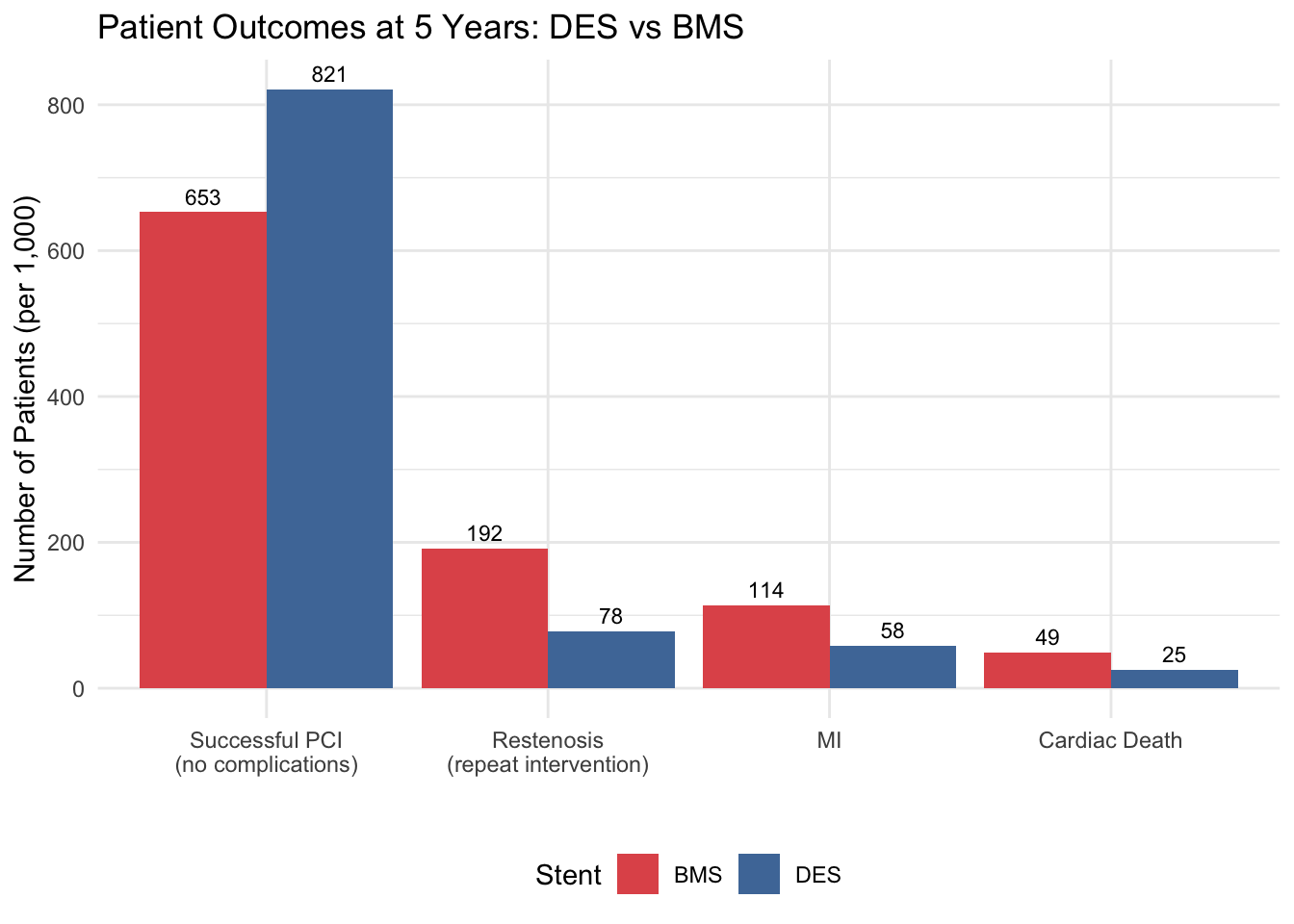
TipCount first, calculate later
This is a deliberate discipline. By counting pathway populations before attaching costs or utilities, you can verify the tree logic independently. Do the numbers add up to 1,000? They should. If not, you have a bug in your tree.
7. Cost Vectors — Attach Costs to Each Pathway
Now we multiply: pathway count × unit cost for each cost component. We build the total cost from pieces, so you can see exactly what drives the expense.
Code
# Discount factor for summing over years
discount_factor <- sum(1 / (1 + discount_rate)^(0:(time_horizon - 1)))

# ============================================================
# DES ARM — Cost components
# ============================================================

# 1. Initial PCI + stent (successful patients get stent; failures get CABG)
cost_initial_des <- des_success * (cost_procedure + cost_des_stent) +
                    des_failure * cost_cabg

# 2. Medications: Year 1 DAPT + annual follow-up (discounted)
cost_medication_des <- n_cohort * cost_dapt_des_annual +
                       n_cohort * cost_followup_annual * discount_factor

# 3. Restenosis management (weighted: 80% repeat PCI, 20% CABG)
cost_restenosis_des <- des_restenosis * (
  (1 - p_cabg_if_restenosis) * cost_repeat_pci +
  p_cabg_if_restenosis * cost_cabg
)

# 4. MACE management
cost_mace_des <- des_mi * cost_mi_management +
                 des_cardiac_death * cost_cardiac_death

# TOTAL
total_cost_des <- cost_initial_des + cost_medication_des +
                  cost_restenosis_des + cost_mace_des

# ============================================================
# BMS ARM — Cost components
# ============================================================
cost_initial_bms <- bms_success * (cost_procedure + cost_bms_stent) +
                    bms_failure * cost_cabg

cost_medication_bms <- n_cohort * cost_dapt_bms_annual +
                       n_cohort * cost_followup_annual * discount_factor

cost_restenosis_bms <- bms_restenosis * (
  (1 - p_cabg_if_restenosis) * cost_repeat_pci +
  p_cabg_if_restenosis * cost_cabg
)

cost_mace_bms <- bms_mi * cost_mi_management +
                 bms_cardiac_death * cost_cardiac_death

total_cost_bms <- cost_initial_bms + cost_medication_bms +
                  cost_restenosis_bms + cost_mace_bms

# --- Clean summary as a table ---
fmt <- function(x) paste0("₹", format(round(x), big.mark = ","))

cost_summary <- data.frame(
  Component = c("Initial PCI + Stent", "Medications (5 yr)",
                "Restenosis management", "MACE management",
                "**TOTAL (cohort)**", "**Per patient**"),
  DES = c(fmt(cost_initial_des), fmt(cost_medication_des),
          fmt(cost_restenosis_des), fmt(cost_mace_des),
          fmt(total_cost_des), fmt(total_cost_des / n_cohort)),
  BMS = c(fmt(cost_initial_bms), fmt(cost_medication_bms),
          fmt(cost_restenosis_bms), fmt(cost_mace_bms),
          fmt(total_cost_bms), fmt(total_cost_bms / n_cohort))
)

kable(cost_summary, col.names = c("Cost Component", "DES", "BMS"),
      caption = "5-year cost summary: DES vs BMS",
align = c("l", "r", "r"))| Cost Component | DES | BMS |
|---|---|---|
| Initial PCI + Stent | ₹161,665,010 | ₹135,465,280 |
| Medications (5 yr) | ₹31,585,492 | ₹26,585,492 |
| Restenosis management | ₹15,054,400 | ₹37,248,000 |
| MACE management | ₹12,869,960 | ₹25,296,000 |
| TOTAL (cohort) | ₹221,174,862 | ₹224,594,772 |
| Per patient | ₹221,175 | ₹224,595 |
Code
library(tidyr)

cost_breakdown <- data.frame(
  Category = c("Initial PCI + Stent", "Medications (5yr)", "Restenosis Mgmt", "MACE Mgmt"),
  DES = c(cost_initial_des, cost_medication_des, cost_restenosis_des, cost_mace_des) / n_cohort,
  BMS = c(cost_initial_bms, cost_medication_bms, cost_restenosis_bms, cost_mace_bms) / n_cohort
)

cost_long <- pivot_longer(cost_breakdown, cols = c(DES, BMS),
                          names_to = "Stent", values_to = "Cost")

ggplot(cost_long, aes(x = Stent, y = Cost, fill = Category)) +
  geom_col(position = "stack") +
  scale_fill_manual(values = c("Initial PCI + Stent" = "#4e79a7",
                                "Medications (5yr)" = "pink",
                                "Restenosis Mgmt" = "#f28e2b",
                                "MACE Mgmt" = "#e15759")) +
  labs(x = "Stent Type", y = "Cost per Patient (₹)",
       title = "5-Year Cost Breakdown: DES vs BMS",
       subtitle = "Indian NPPA ceiling prices (2025)") +
  theme_minimal() +
  theme(legend.position = "bottom")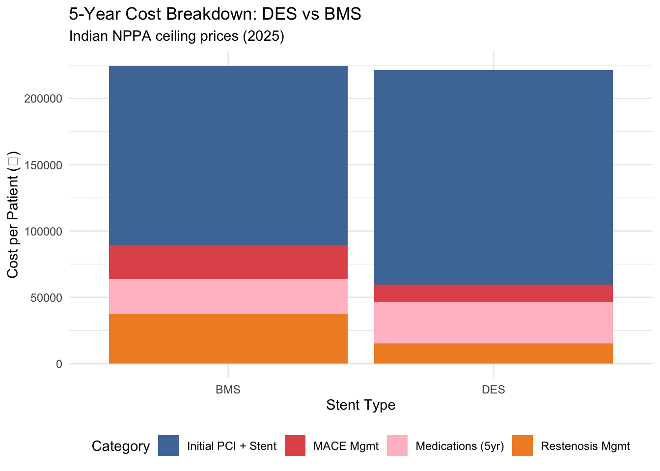
NoteThe cost story
DES costs more upfront (₹28,240 more per stent), but look at the restenosis and MACE management bars — BMS generates far more downstream costs. Whether DES ends up cheaper overall depends on the balance between these components.
8. QALY Vectors — Attach Utilities to Each Pathway
Same logic: pathway count × utility weight × time. Each patient group accumulates QALYs at a rate determined by their health state.
Code
# ============================================================
# DES ARM — QALY components
# ============================================================

# Patients who are well (no restenosis, no MACE) — best outcome
qaly_des_well <- des_no_mace_no_restenosis * utility_well_post_pci * time_horizon

# Restenosis but recovered (no subsequent MACE)
# 6 months unwell pre-intervention, then recovered for remaining years
qaly_des_restenosis_ok <- des_no_mace_from_restenosis *
  (utility_well_post_pci * 0.5 + utility_restenosis_recovered * (time_horizon - 0.5))

# MI survivors
# ~2 years well before MI, then reduced utility for remaining years
qaly_des_mi <- des_mi *
  (utility_well_post_pci * 2 + utility_post_mi * (time_horizon - 2))

# Cardiac death (assumed at midpoint of follow-up)
qaly_des_death <- des_cardiac_death * utility_well_post_pci * (time_horizon / 2)

# Procedural failures (→ CABG, assumed similar to restenosis recovery)
qaly_des_failure <- des_failure * utility_restenosis_recovered * time_horizon

# TOTAL
total_qaly_des <- qaly_des_well + qaly_des_restenosis_ok +
                  qaly_des_mi + qaly_des_death + qaly_des_failure

# ============================================================
# BMS ARM — QALY components
# ============================================================
qaly_bms_well <- bms_no_mace_no_restenosis * utility_well_post_pci * time_horizon

qaly_bms_restenosis_ok <- bms_no_mace_from_restenosis *
  (utility_well_post_pci * 0.5 + utility_restenosis_recovered * (time_horizon - 0.5))

qaly_bms_mi <- bms_mi *
  (utility_well_post_pci * 2 + utility_post_mi * (time_horizon - 2))

qaly_bms_death <- bms_cardiac_death * utility_well_post_pci * (time_horizon / 2)

qaly_bms_failure <- bms_failure * utility_restenosis_recovered * time_horizon

total_qaly_bms <- qaly_bms_well + qaly_bms_restenosis_ok +
                  qaly_bms_mi + qaly_bms_death + qaly_bms_failure

# --- Clean summary as a table ---
qaly_summary <- data.frame(
  Component = c("Well (no complications)", "Restenosis recovered",
                "MI survivors", "Cardiac death", "Procedural failure",
                "**TOTAL (cohort)**", "**Per patient**"),
  DES = c(round(qaly_des_well, 1), round(qaly_des_restenosis_ok, 1),
          round(qaly_des_mi, 1), round(qaly_des_death, 1),
          round(qaly_des_failure, 1),
          round(total_qaly_des, 1), round(total_qaly_des / n_cohort, 3)),
  BMS = c(round(qaly_bms_well, 1), round(qaly_bms_restenosis_ok, 1),
          round(qaly_bms_mi, 1), round(qaly_bms_death, 1),
          round(qaly_bms_failure, 1),
          round(total_qaly_bms, 1), round(total_qaly_bms / n_cohort, 3))
)

kable(qaly_summary, col.names = c("Patient Group", "DES (QALYs)", "BMS (QALYs)"),
      caption = "5-year QALY summary: DES vs BMS",
align = c("l", "r", "r"))| Patient Group | DES (QALYs) | BMS (QALYs) |
|---|---|---|
| Well (no complications) | 3489.300 | 2774.400 |
| Restenosis recovered | 259.600 | 566.600 |
| MI survivors | 212.100 | 417.000 |
| Cardiac death | 52.900 | 104.000 |
| Procedural failure | 117.000 | 156.000 |
| TOTAL (cohort) | 4130.900 | 4018.100 |
| Per patient | 4.131 | 4.018 |
9. The ICER — Defining and Calculating
The Incremental Cost-Effectiveness Ratio is the core metric of HTA. Let’s define it as a function — because we will reuse it many times.
Code
# === ICER FUNCTION ===
calc_icer <- function(cost_new, cost_old, qaly_new, qaly_old) {
  inc_cost <- cost_new - cost_old
  inc_qaly <- qaly_new - qaly_old
  icer     <- inc_cost / inc_qaly
  list(inc_cost = inc_cost, inc_qaly = inc_qaly, icer = icer)
}

# Apply to our results
result <- calc_icer(
  cost_new = total_cost_des, cost_old = total_cost_bms,
  qaly_new = total_qaly_des, qaly_old = total_qaly_bms
)

# --- Interpret against WTP thresholds ---
wtp_1gdp <- 170000    # ~1× GDP per capita India
wtp_3gdp <- 510000    # ~3× GDP per capita

interpretation <- if (result$inc_cost < 0 && result$inc_qaly > 0) {
  "DES is **DOMINANT** (less costly AND more effective)"
} else if (result$inc_cost > 0 && result$inc_qaly < 0) {
  "DES is **DOMINATED** (more costly AND less effective)"
} else if (result$inc_cost < 0 && result$inc_qaly < 0) {
  "DES is **dominated on cost** but less effective (rare dominance scenario)"
} else if (result$inc_cost > 0 && result$inc_qaly > 0) {
  if (result$icer < wtp_1gdp) {
    "DES is **HIGHLY cost-effective** (ICER < 1× GDP per capita)"
  } else if (result$icer < wtp_3gdp) {
    "DES is **cost-effective** (ICER < 3× GDP per capita)"
  } else {
    "DES is **NOT cost-effective** at conventional WTP thresholds"
  }
} else {
  "Undefined scenario — check calculations"
}

# Display as a clean summary table
icer_table <- data.frame(
  Metric = c("Incremental cost (DES − BMS)",
             "Incremental QALYs (DES − BMS)",
             "ICER",
             "Interpretation"),
  Value = c(paste0("₹", format(round(result$inc_cost), big.mark = ",")),
            round(result$inc_qaly, 2),
            paste0("₹", format(round(result$icer), big.mark = ","), " per QALY"),
            interpretation)
)

kable(icer_table, col.names = c("", ""),
      caption = "Incremental cost-effectiveness: DES vs BMS",
align = c("l", "l"))| Incremental cost (DES − BMS) | ₹-3,419,910 |
| Incremental QALYs (DES − BMS) | 112.86 |
| ICER | ₹-30,302 per QALY |
| Interpretation | DES is DOMINANT (less costly AND more effective) |
Net Monetary Benefit (NMB) Analysis
The Net Monetary Benefit offers an alternative perspective on cost-effectiveness. Rather than expressing value as a ratio, NMB converts QALYs into monetary units using the WTP threshold, then subtracts costs. A positive NMB means the intervention is worth adopting; a negative NMB means rejection.
Formula: NMB = (WTP × QALYs) − Cost
Code
# Define WTP thresholds
wtp_india <- 170000    # 1× GDP per capita (₹)

# Per-patient costs and QALYs (from earlier sections)
cost_per_patient_des <- total_cost_des / n_cohort
cost_per_patient_bms <- total_cost_bms / n_cohort
qaly_per_patient_des <- total_qaly_des / n_cohort
qaly_per_patient_bms <- total_qaly_bms / n_cohort

# Calculate NMB for each strategy
nmb_des <- wtp_india * qaly_per_patient_des - cost_per_patient_des
nmb_bms <- wtp_india * qaly_per_patient_bms - cost_per_patient_bms

# Incremental NMB (ΔNMB)
inc_nmb <- nmb_des - nmb_bms

# Decision rule
nmb_decision <- if (inc_nmb > 0) {
  "**ADOPT DES** — positive incremental NMB"
} else if (inc_nmb < 0) {
  "**REJECT DES** — negative incremental NMB (stick with BMS)"
} else {
  "**INDIFFERENT** — ΔNMB = 0"
}

# Display as table
nmb_table <- data.frame(
  Metric = c("NMB: DES per patient",
             "NMB: BMS per patient",
             "Incremental NMB (ΔNMB)",
             "Decision"),
  Value = c(paste0("₹", format(round(nmb_des), big.mark = ",")),
            paste0("₹", format(round(nmb_bms), big.mark = ",")),
            paste0("₹", format(round(inc_nmb), big.mark = ",")),
            nmb_decision)
)

kable(nmb_table, col.names = c("", ""),
      caption = paste0("Net Monetary Benefit at WTP = ₹", format(wtp_india, big.mark = ","), "/QALY"),
align = c("l", "l"))| NMB: DES per patient | ₹481,081 |
| NMB: BMS per patient | ₹458,475 |
| Incremental NMB (ΔNMB) | ₹22,606 |
| Decision | ADOPT DES — positive incremental NMB |
NoteNMB as a decision tool
NMB and ICER will always agree on the direction of the decision — if DES is cost-effective by ICER, ΔNMB will be positive. But NMB has a practical advantage: it’s in currency units, not a ratio. Policy makers can directly ask: “How much net health gain does this intervention create, valued in monetary terms?” A health system with a fixed budget might adopt the intervention that maximizes total NMB for all patients, not just the one with the lowest ICER.
Code
# NNT — a clinical translation of the ICER
nnt_restenosis <- round(1 / (p_restenosis_bms - p_restenosis_des))
nnt_mace <- round(1 / ((bms_total_mace - des_total_mace) / n_cohort))

nnt_data <- data.frame(
  Outcome = c("Avoid 1\nRestenosis", "Avoid 1\nMACE Event"),
  NNT = c(nnt_restenosis, nnt_mace)
)

ggplot(nnt_data, aes(x = Outcome, y = NNT, fill = Outcome)) +
  geom_col(show.legend = FALSE) +
  geom_text(aes(label = paste0("NNT = ", NNT)), vjust = -0.5, size = 4, fontface = "bold") +
  scale_fill_manual(values = c("#4e79a7", "#e15759")) +
  labs(x = "", y = "Number Needed to Treat",
       title = "How Many Patients Need DES to Prevent One Event?",
       subtitle = "Compared to BMS over 5-year horizon") +
  theme_minimal() +
  expand_limits(y = c(0, max(nnt_data$NNT) * 1.2))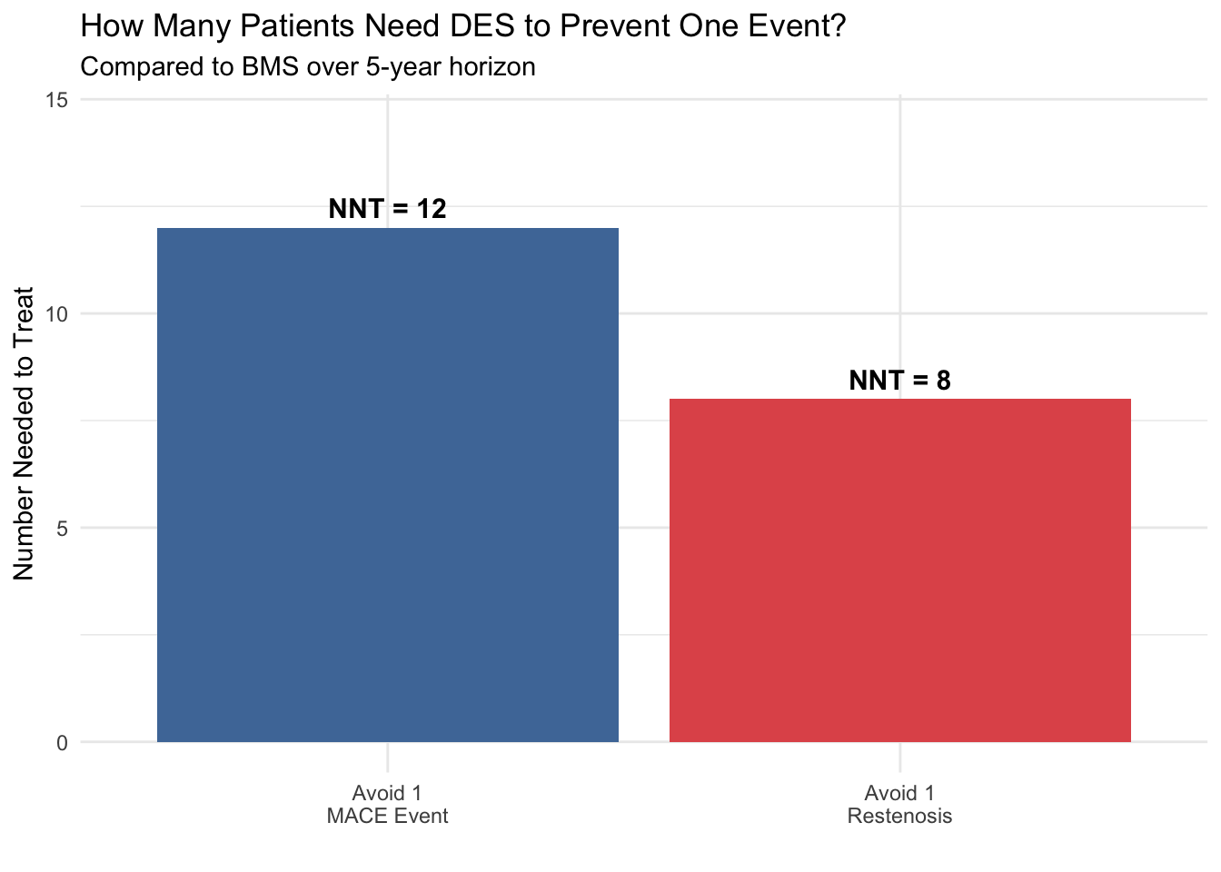
10. Visualising the Results
Code
outcomes <- data.frame(
  Outcome = rep(c("Restenosis", "MI", "Cardiac Death"), 2),
  Stent = rep(c("DES", "BMS"), each = 3),
  Count = c(round(des_restenosis), round(des_mi), round(des_cardiac_death),
            round(bms_restenosis), round(bms_mi), round(bms_cardiac_death))
)

ggplot(outcomes, aes(x = Outcome, y = Count, fill = Stent)) +
  geom_col(position = "dodge") +
  geom_text(aes(label = Count), position = position_dodge(width = 0.9), vjust = -0.5, size = 3) +
  scale_fill_manual(values = c("DES" = "#4e79a7", "BMS" = "#e15759")) +
  labs(x = "", y = "Number of Patients (per 1,000)",
       title = "Clinical Outcomes: DES vs BMS at 5 Years") +
  theme_minimal() +
  theme(legend.position = "bottom")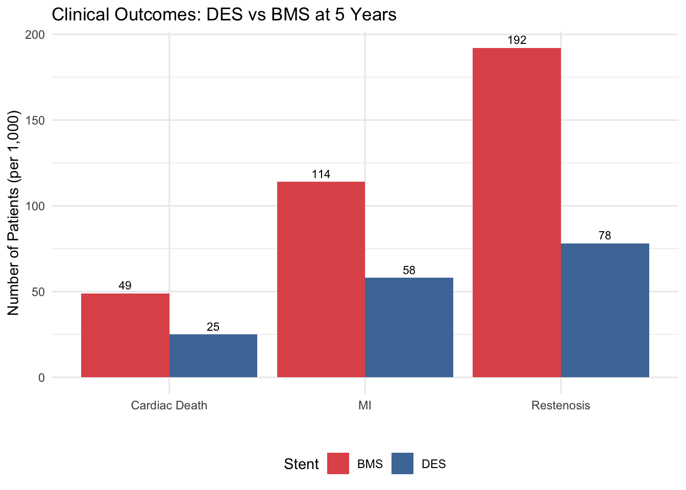
11. What Should Keep You Up at Night
We have an ICER. The model says DES is cost-effective. But how confident are you?
Every number in this model is a point estimate — a single “best guess.” In reality, each parameter carries uncertainty. The questions below expose why a single ICER is not enough, and why we need sensitivity analysis (our next sessions).
But first — wrapping the model in a function
Look back at Sections 6–9. You wrote about 80 lines of R code to get from parameters to ICER. Now imagine you want to ask: “What if the restenosis rate were 12% instead of 20%?” Would you copy-paste those 80 lines and change one number? What about testing 10 different restenosis rates? 100?
This is where functions transform your workflow. A function wraps your entire model into a single reusable command. You change one input, call the function, and get the answer. No copy-paste, no errors from forgetting to update a line.
TipFunctions = Reusable models
Remember from Session 2 (R Orientation): a function takes inputs, does something, and returns outputs. In HTA, your model is a function — it takes parameters and returns costs, QALYs, and an ICER. Wrapping it this way is not just good coding practice; it is essential for sensitivity analysis, where you will call this function hundreds or thousands of times with different inputs.
Code
# ============================================================
# THE MODEL AS A FUNCTION
# ============================================================
# Everything from Sections 6–9, wrapped so we can reuse it.
# Default values = our base case. Change any input to explore.

run_model <- function(p_rest_des = 0.08, p_rest_bms = 0.20,
                      c_des = 38933, c_bms = 10693,
                      u_well = 0.85, u_rest = 0.78, u_mi = 0.65) {

  des_s   <- n_cohort * p_success_des
  des_r   <- des_s * p_rest_des
  des_nr  <- des_s * (1 - p_rest_des)
  des_mac <- des_r * p_mace_des_restenosis + des_nr * p_mace_des_no_restenosis
  des_m   <- des_mac * p_mi_given_mace
  des_d   <- des_mac * p_cardiac_death_given_mace

  bms_s   <- n_cohort * p_success_bms
  bms_r   <- bms_s * p_rest_bms
  bms_nr  <- bms_s * (1 - p_rest_bms)
  bms_mac <- bms_r * p_mace_bms_restenosis + bms_nr * p_mace_bms_no_restenosis
  bms_m   <- bms_mac * p_mi_given_mace
  bms_d   <- bms_mac * p_cardiac_death_given_mace

  df <- sum(1 / (1 + discount_rate)^(0:(time_horizon - 1)))

  tc_des <- des_s * (cost_procedure + c_des) + (n_cohort - des_s) * cost_cabg +
            n_cohort * cost_dapt_des_annual + n_cohort * cost_followup_annual * df +
            des_r * ((1 - p_cabg_if_restenosis) * cost_repeat_pci + p_cabg_if_restenosis * cost_cabg) +
            des_m * cost_mi_management + des_d * cost_cardiac_death

  tc_bms <- bms_s * (cost_procedure + c_bms) + (n_cohort - bms_s) * cost_cabg +
            n_cohort * cost_dapt_bms_annual + n_cohort * cost_followup_annual * df +
            bms_r * ((1 - p_cabg_if_restenosis) * cost_repeat_pci + p_cabg_if_restenosis * cost_cabg) +
            bms_m * cost_mi_management + bms_d * cost_cardiac_death

  tq_des <- (des_nr - des_nr * p_mace_des_no_restenosis) * u_well * time_horizon +
            (des_r - des_r * p_mace_des_restenosis) * (u_well * 0.5 + u_rest * (time_horizon - 0.5)) +
            des_m * (u_well * 2 + u_mi * 3) +
            des_d * u_well * (time_horizon / 2) +
            (n_cohort - des_s) * u_rest * time_horizon

  tq_bms <- (bms_nr - bms_nr * p_mace_bms_no_restenosis) * u_well * time_horizon +
            (bms_r - bms_r * p_mace_bms_restenosis) * (u_well * 0.5 + u_rest * (time_horizon - 0.5)) +
            bms_m * (u_well * 2 + u_mi * 3) +
            bms_d * u_well * (time_horizon / 2) +
            (n_cohort - bms_s) * u_rest * time_horizon

  list(cost_des = tc_des, cost_bms = tc_bms,
       qaly_des = tq_des, qaly_bms = tq_bms,
       icer = (tc_des - tc_bms) / (tq_des - tq_bms))
}
Now we can explore “what if” questions with a single line of code. Watch how easy it becomes.
Question 1: What if restenosis rates are different?
The restenosis rate differential is the biggest clinical driver. We used 8% for DES and 20% for BMS. But what if newer BMS perform better — say 12% restenosis?
Code
# One line each — that's the power of a function
base <- run_model()                       # base case
alt  <- run_model(p_rest_bms = 0.12)      # what if BMS improves?

kable(data.frame(
  Scenario = c("Base case (DES 8% vs BMS 20%)",
               "BMS restenosis drops to 12%"),
  ICER = c(paste0("₹", format(round(base$icer), big.mark = ",")),
           paste0("₹", format(round(alt$icer), big.mark = ",")))
), col.names = c("Scenario", "ICER (₹/QALY)"),
  caption = "How restenosis rates change the conclusion",
align = c("l", "r"))| Scenario | ICER (₹/QALY) |
|---|---|
| Base case (DES 8% vs BMS 20%) | ₹-30,302 |
| BMS restenosis drops to 12% | ₹146,310 |
Warning
The ICER changes dramatically with one parameter. How confident are you in the 20% estimate? This is exactly what Deterministic Sensitivity Analysis (DSA) addresses — varying one parameter at a time to see which ones matter most.
Questions to carry forward
The restenosis example above is just the beginning. Here are questions we cannot answer with a single ICER — and each one points to a method we will learn in the next sessions:
At what DES price does it stop being worth it? NPPA ceilings can be revised. Costs rise with inflation. There must be a price beyond which DES is no longer cost-effective — but what is it? → Threshold analysis / DSA
What if ALL uncertain parameters vary at once? We used point estimates throughout. But every probability, cost, and utility has a range. What does the ICER look like when everything varies simultaneously? → Probabilistic Sensitivity Analysis (PSA)
“How confident are you that DES is cost-effective?” A policy maker won’t accept a single number. They want a probability. You cannot answer this with one ICER — you need a distribution of ICERs. → Cost-Effectiveness Acceptability Curve (CEAC)
What about Indian utility values? We flagged that our utility weights come from international literature. If Indian patients experience different quality of life, the entire conclusion could shift. Is it worth investing in a local EQ-5D study? → Value of Information (VOI) analysis
ImportantThe bridge to next sessions
A single ICER is a starting point, not the answer. The real answer is: how robust is this conclusion to the things we don’t know? That is what sensitivity analysis provides, and it is exactly what we will build next — using the run_model() function you just created.
Key References
- NPPA India. Revised ceiling prices for coronary stents (2025).
- Bangalore S et al. (2012). Short- and long-term outcomes with DES and BMS. Circulation.
- Kaul U et al. (2017). India and the coronary stent market. Circulation.
- PMC (2010). Comparative study of restenosis rates in BMS and DES — Indian data.
- NEJM (2016). Drug-eluting or bare-metal stents for coronary artery disease.
- Sullivan PW et al. (2011). Catalog of EQ-5D scores for the United Kingdom. Medical Decision Making.
→ Next session: We’ll take this exact model and systematically vary every parameter — first one at a time (DSA), then all at once (PSA).