---
title: "Session 5: 4-State Markov Model — Chronic Kidney Disease"
subtitle: "Early screening and ACE-inhibitor intervention vs standard care"
format:
html:
toc: true
code-fold: show
code-tools: true
---
## 1. The Clinical Question
Chronic kidney disease (CKD) affects approximately 17% of the Indian population, with about 6% having stage 3 or worse. Most patients in India present late — over 50% are first seen when eGFR is already below 15 ml/min (stage 5), by which point dialysis or transplantation is needed at enormous cost.
**The HTA question:** Is early population-based screening for CKD followed by ACE-inhibitor therapy cost-effective compared to standard care (where CKD is detected only when symptomatic or incidental)?
This is a **Markov cohort model** — the most common model type for chronic diseases that progress through stages over time.
## 2. What Is a Markov Model?
A Markov model tracks a **cohort** of patients through defined **health states** over multiple **time cycles** (usually years). At each cycle, patients can:
- Stay in their current state
- Move to a worse state (progression)
- Move to a better state (rare in CKD, but possible with treatment)
- Die
The movement between states is governed by **transition probabilities**. These probabilities are the heart of the model.
## 3. Our 4-State Model
```{r}
#| label: fig-ckd-states
#| echo: true
#| fig-cap: "CKD Markov model: health states and transitions"
library(DiagrammeR)

grViz("
digraph ckd_markov {
  graph [rankdir=LR, bgcolor='transparent', fontname='Helvetica', nodesep=0.8]
  node [fontname='Helvetica', fontsize=11, style='filled,rounded', shape=box]

  E [label='Early CKD\n(Stage 1-2)\neGFR ≥ 60', fillcolor='#59a14f', fontcolor='white', width=1.8]
  M [label='Moderate CKD\n(Stage 3)\neGFR 30-59', fillcolor='#f28e2b', fontcolor='white', width=1.8]
  A [label='Advanced CKD\n/ Dialysis\n(Stage 4-5)', fillcolor='#e15759', fontcolor='white', width=1.8]
  D [label='Death', fillcolor='#76b7b2', fontcolor='white', shape=doublecircle, width=1.2]

  E -> M [label='p_12', fontsize=10]
  M -> A [label='p_23', fontsize=10]
  E -> D [label='p_1d', fontsize=10]
  M -> D [label='p_2d', fontsize=10]
  A -> D [label='p_3d', fontsize=10]

  E -> E [label='stay', style=dashed, fontsize=9]
  M -> M [label='stay', style=dashed, fontsize=9]
  A -> A [label='stay', style=dashed, fontsize=9]
}
")
```
The four states are:
1. **Early CKD (Stage 1-2):** eGFR ≥60, often asymptomatic. Managed with lifestyle modification and renoprotective drugs.
2. **Moderate CKD (Stage 3):** eGFR 30-59. Requires specialist referral, medication optimisation.
3. **Advanced CKD / Dialysis (Stage 4-5):** eGFR <30. Requires dialysis or transplantation.
4. **Death:** Absorbing state — patients cannot leave.
## 4. Model Parameters
```{r}
#| label: parameters
#| echo: true
library(knitr)

# ============================================================
# MODEL PARAMETERS — CKD Markov Model
# ============================================================

# --- Cohort ---
n_cohort <- 10000   # Cohort of 10,000 patients with early CKD
n_cycles <- 20      # 20-year time horizon
cycle_length <- 1   # Annual cycles

# --- Starting Distribution ---
# All patients start in Early CKD (detected through screening)
state_names <- c("Early CKD", "Moderate CKD", "Advanced/Dialysis", "Death")
n_states <- length(state_names)

# --- Annual Transition Probabilities: STANDARD CARE ---
# Source: Adapted from international CKD progression literature
# (Go et al. 2004 NEJM; Kerr et al. 2012; SEEK study India)
# Adjusted for Indian demographics (younger onset, higher diabetes burden)

# From Early CKD (Stage 1-2)
p_12_standard <- 0.10   # Early → Moderate (annual)
p_1d_standard <- 0.02   # Early → Death (background + CKD-related)

# From Moderate CKD (Stage 3)
p_23_standard <- 0.12   # Moderate → Advanced (annual)
p_2d_standard <- 0.04   # Moderate → Death

# From Advanced CKD / Dialysis (Stage 4-5)
p_3d_standard <- 0.15   # Advanced → Death (annual)
# Source: Indian dialysis mortality ~15-25% annually
# (Rajapurkar et al. 2012; Indian CKD Registry)

# --- Costs (₹ per year) ---
# Source: Indian hospital data; PMJAY package rates; Jeloka et al. 2007;
#         Inside CKD India projections (Lancet eClinicalMedicine 2024)

# State costs (annual)
cost_early    <- 12000    # OPD visits, basic labs, lifestyle counselling
cost_moderate <- 45000    # Specialist visits, medications, frequent labs
cost_advanced <- 350000   # Dialysis (2-3 sessions/week at public hospital rates)
cost_death    <- 0

# Intervention-specific costs
cost_screening  <- 500     # One-time population screening cost per person
cost_ace_annual <- 6000    # ACE-inhibitor + monitoring (generic enalapril/ramipril)

# --- Utility Weights (annual QALYs) ---
# Source: Adapted from Gorodetskaya et al. 2005; Tajima et al. 2010
# Indian EQ-5D data limited; disclaimer applies
utility_early    <- 0.85
utility_moderate <- 0.72
utility_advanced <- 0.55   # Dialysis significantly reduces quality of life
utility_death    <- 0.00

# --- Discount Rate ---
discount_rate <- 0.03  # 3% annual for both costs and QALYs

# --- WTP Threshold ---
wtp_india <- 170000  # ~1x GDP per capita India
```
### Parameter summary
```{r}
#| label: param-summary
#| echo: true
# Display parameters as a clean table
param_table <- data.frame(
  Parameter = c("Cohort size", "Time horizon", "Discount rate",
                "p(Early→Moderate)", "p(Early→Death)",
                "p(Moderate→Advanced)", "p(Moderate→Death)",
                "p(Advanced→Death)",
                "Cost: Early CKD", "Cost: Moderate CKD",
                "Cost: Advanced/Dialysis", "Cost: Screening (one-time)",
                "Cost: ACE-inhibitor (annual)",
                "Utility: Early", "Utility: Moderate",
                "Utility: Advanced", "Utility: Death"),
  Value = c("10,000", "20 years", "3%",
            "0.10", "0.02", "0.12", "0.04", "0.15",
            "₹12,000", "₹45,000", "₹3,50,000", "₹500", "₹6,000",
            "0.85", "0.72", "0.55", "0.00"),
  Source = c("Assumption", "Standard for chronic disease", "Indian HTA guidelines",
             "Go 2004; SEEK India", "Background + CKD-related",
             "Go 2004; Kerr 2012", "CKD-related excess mortality",
             "Indian CKD Registry; Rajapurkar 2012",
             "PMJAY rates", "Specialist care estimates",
             "Public hospital dialysis", "Population screening", "Generic enalapril",
             "Gorodetskaya 2005", "Gorodetskaya 2005",
             "Tajima 2010; Indian EQ-5D limited", "Convention")
)

kable(param_table, align = "llr",
      caption = "Model parameters with sources")
```
## 5. Hazard Ratio to Probability Conversion
Clinical trials report treatment effects as **hazard ratios** (HR). An HR of 0.66 means the ACE-inhibitor reduces the *rate* of progression by 34%. But our Markov model needs *probabilities*, not rates. How do we convert?
The key relationship between probability ($p$) and rate ($r$) over one cycle is:
$$p = 1 - e^{-r}$$
And the reverse:
$$r = -\ln(1 - p)$$
To apply a hazard ratio, we: (1) convert the baseline probability to a rate, (2) multiply the rate by HR, and (3) convert back to a probability. This simplifies to:
$$p_{\text{intervention}} = 1 - (1 - p_{\text{standard}})^{HR}$$
```{r}
#| label: hr-conversion
#| echo: true
# --- Treatment Effect: HR = 0.66 ---
treatment_effect_hr <- 0.66

# Step-by-step conversion for Early → Moderate
rate_12 <- -log(1 - p_12_standard)                     # Step 1: prob → rate
rate_12_int <- rate_12 * treatment_effect_hr            # Step 2: apply HR
p_12_intervention <- 1 - exp(-rate_12_int)              # Step 3: rate → prob

# This is mathematically equivalent to the shortcut:
p_12_shortcut <- 1 - (1 - p_12_standard)^treatment_effect_hr

# Verify they match
kable(data.frame(
  Transition = c("Early → Moderate", "Moderate → Advanced"),
  Standard = c(p_12_standard, p_23_standard),
  `Step-by-step` = c(p_12_intervention, 1 - exp(-(-log(1 - p_23_standard)) * treatment_effect_hr)),
  Shortcut = c(p_12_shortcut, 1 - (1 - p_23_standard)^treatment_effect_hr),
  check.names = FALSE
), digits = 6, caption = "HR → probability conversion: both methods agree")
# Use the shortcut going forward
p_12_intervention <- 1 - (1 - p_12_standard)^treatment_effect_hr
p_23_intervention <- 1 - (1 - p_23_standard)^treatment_effect_hr

# Mortality not directly affected by ACE-inhibitor
p_1d_intervention <- p_1d_standard
p_2d_intervention <- p_2d_standard
p_3d_intervention <- p_3d_standard
```
::: {.callout-warning}
## Common Mistake
You **cannot** simply multiply the probability by the HR: `0.10 × 0.66 = 0.066` is wrong. That approach underestimates the true intervention probability (correct value: `r round(p_12_intervention, 4)`). The error grows larger with higher baseline probabilities. Always use the rate-based conversion.
:::
## 6. Building the Transition Matrices
A **transition matrix** is a table where each row represents the current state and each column represents where patients can go. Each row must sum to 1.0 (everyone goes somewhere).
### Step 1: Create the scaffold
```{r}
#| label: matrix-scaffold
#| echo: true
# Start with an empty 4×4 matrix of zeros
tm_standard <- matrix(0, nrow = n_states, ncol = n_states,
                      dimnames = list(state_names, state_names))

# At this point, every cell is 0:
kable(tm_standard, digits = 2,
      caption = "Step 1: Empty scaffold — all zeros")
```
### Step 2: Populate with transition probabilities
You can address cells by **state name** (clearer, self-documenting) or by **row/column number** (shorter). Both are equivalent:
```{r}
#| label: matrix-populate
#| echo: true
# --- Method A: State-name indexing (recommended for clarity) ---
# From Early CKD
tm_standard["Early CKD", "Moderate CKD"] <- p_12_standard       # progression
tm_standard["Early CKD", "Death"]        <- p_1d_standard       # mortality
tm_standard["Early CKD", "Early CKD"]    <- 1 - p_12_standard - p_1d_standard  # stay

# From Moderate CKD
tm_standard["Moderate CKD", "Advanced/Dialysis"] <- p_23_standard
tm_standard["Moderate CKD", "Death"]             <- p_2d_standard
tm_standard["Moderate CKD", "Moderate CKD"]      <- 1 - p_23_standard - p_2d_standard

# From Advanced/Dialysis
tm_standard["Advanced/Dialysis", "Death"]             <- p_3d_standard
tm_standard["Advanced/Dialysis", "Advanced/Dialysis"]  <- 1 - p_3d_standard

# Death is absorbing
tm_standard["Death", "Death"] <- 1

# --- Method B: Numeric indexing (equivalent) ---
# tm_standard[1, 2] <- p_12_standard      # row 1 = Early, col 2 = Moderate
# tm_standard[1, 4] <- p_1d_standard      # row 1 = Early, col 4 = Death
# tm_standard[1, 1] <- 1 - p_12_standard - p_1d_standard
# ... and so on

kable(tm_standard, digits = 4,
      caption = "Standard Care transition matrix — completed")
```
::: {.callout-tip}
## The "Stay" Probability
The diagonal (stay probability) is always **1 minus all outgoing probabilities**. For Early CKD: `1 - 0.10 - 0.02 = 0.88`. A common bug is writing `1 - p_12` and forgetting to subtract `p_1d` — that would make the row sum exceed 1.0.
:::
### Row-sum verification
```{r}
#| label: rowsum-check
#| echo: true
# Every row must sum to exactly 1.0
kable(data.frame(
  State = state_names,
  `Row Sum` = rowSums(tm_standard),
  check.names = FALSE
), caption = "Row-sum check: all rows must equal 1.000")
```
### Intervention matrix
```{r}
#| label: intervention-matrix
#| echo: true
# Build intervention matrix — same structure, different progression rates
tm_intervention <- matrix(0, nrow = n_states, ncol = n_states,
                          dimnames = list(state_names, state_names))

tm_intervention["Early CKD", "Moderate CKD"] <- p_12_intervention
tm_intervention["Early CKD", "Death"]        <- p_1d_intervention
tm_intervention["Early CKD", "Early CKD"]    <- 1 - p_12_intervention - p_1d_intervention

tm_intervention["Moderate CKD", "Advanced/Dialysis"] <- p_23_intervention
tm_intervention["Moderate CKD", "Death"]             <- p_2d_intervention
tm_intervention["Moderate CKD", "Moderate CKD"]      <- 1 - p_23_intervention - p_2d_intervention

tm_intervention["Advanced/Dialysis", "Death"]             <- p_3d_intervention
tm_intervention["Advanced/Dialysis", "Advanced/Dialysis"]  <- 1 - p_3d_intervention

tm_intervention["Death", "Death"] <- 1

kable(tm_intervention, digits = 4,
      caption = "Intervention transition matrix — ACE-inhibitor slows progression")
```
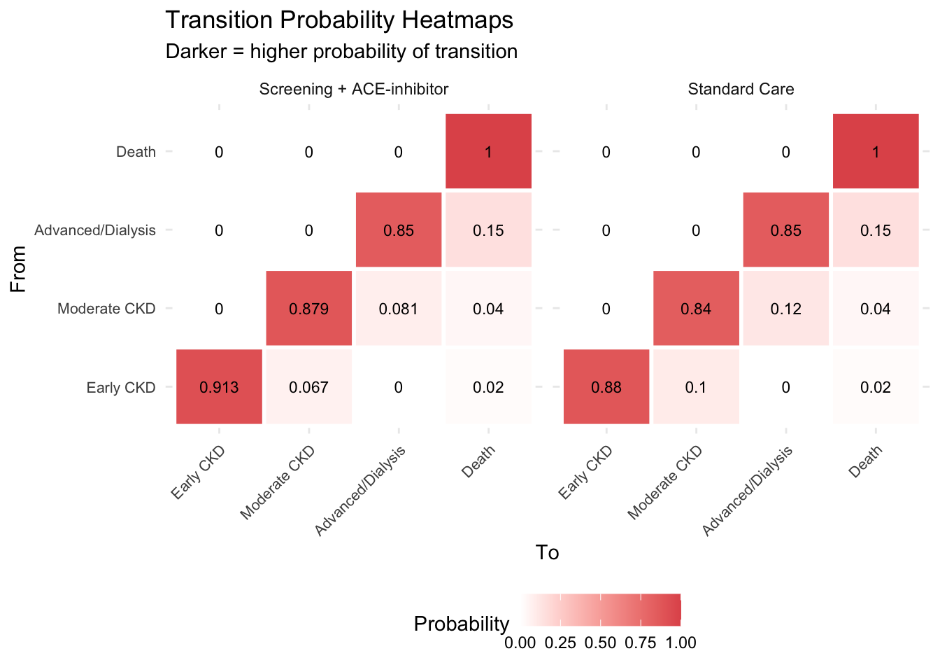
::: {.callout-tip}
## Key Insight: The Matrices
The two matrices differ **only** in the progression probabilities (Early→Moderate and Moderate→Advanced). The treatment slows progression but does not change mortality directly. This is a realistic representation of what ACE-inhibitors do — they buy time, keeping patients in less costly, higher-quality health states for longer.
:::
### Transition matrix heatmap
```{r}
#| label: fig-tm-heatmap
#| echo: true
#| fig-cap: "Transition matrix heatmap — Standard Care vs Intervention"
library(tidyr)
library(ggplot2)
tm_df_std <- as.data.frame(as.table(tm_standard))
names(tm_df_std) <- c("From", "To", "Probability")
tm_df_std$Strategy <- "Standard Care"

tm_df_int <- as.data.frame(as.table(tm_intervention))
names(tm_df_int) <- c("From", "To", "Probability")
tm_df_int$Strategy <- "Screening + ACE-inhibitor"

tm_combined <- rbind(tm_df_std, tm_df_int)

ggplot(tm_combined, aes(x = To, y = From, fill = Probability)) +
  geom_tile(colour = "white", linewidth = 1) +
  geom_text(aes(label = round(Probability, 3)), size = 3) +
  facet_wrap(~Strategy) +
  scale_fill_gradient(low = "white", high = "#e15759") +
  labs(title = "Transition Probability Heatmaps",
       subtitle = "Darker = higher probability of transition") +
  theme_minimal() +
  theme(axis.text.x = element_text(angle = 45, hjust = 1, size = 8),
        axis.text.y = element_text(size = 8),
        legend.position = "bottom")
```
## 7. Matrix Multiplication — How the Simulation Works
The simulation engine is a single line of R: `trace[cycle + 1, ] <- trace[cycle, ] %*% tm`. But what does `%*%` **actually compute**? Let's break it down from first principles.
### The dimension rule: m×n · n×p → m×p
Matrix multiplication is only possible when the **inner dimensions match**. The result takes its rows from the first matrix and columns from the second:
$$\underbrace{A}_{m \times n} \times \underbrace{B}_{n \times p} = \underbrace{C}_{m \times p}$$
In our Markov model, the state vector (1 row × 4 columns) multiplied by the transition matrix (4 rows × 4 columns) gives a new state vector (1 row × 4 columns):
$$\underbrace{\text{trace}}_{1 \times 4} \times \underbrace{\text{TM}}_{4 \times 4} = \underbrace{\text{new trace}}_{1 \times 4}$$
The inner dimension (4 = 4) matches — that's the number of health states. Each element in the result comes from one **dot product** — a row from the left meeting a column from the right.
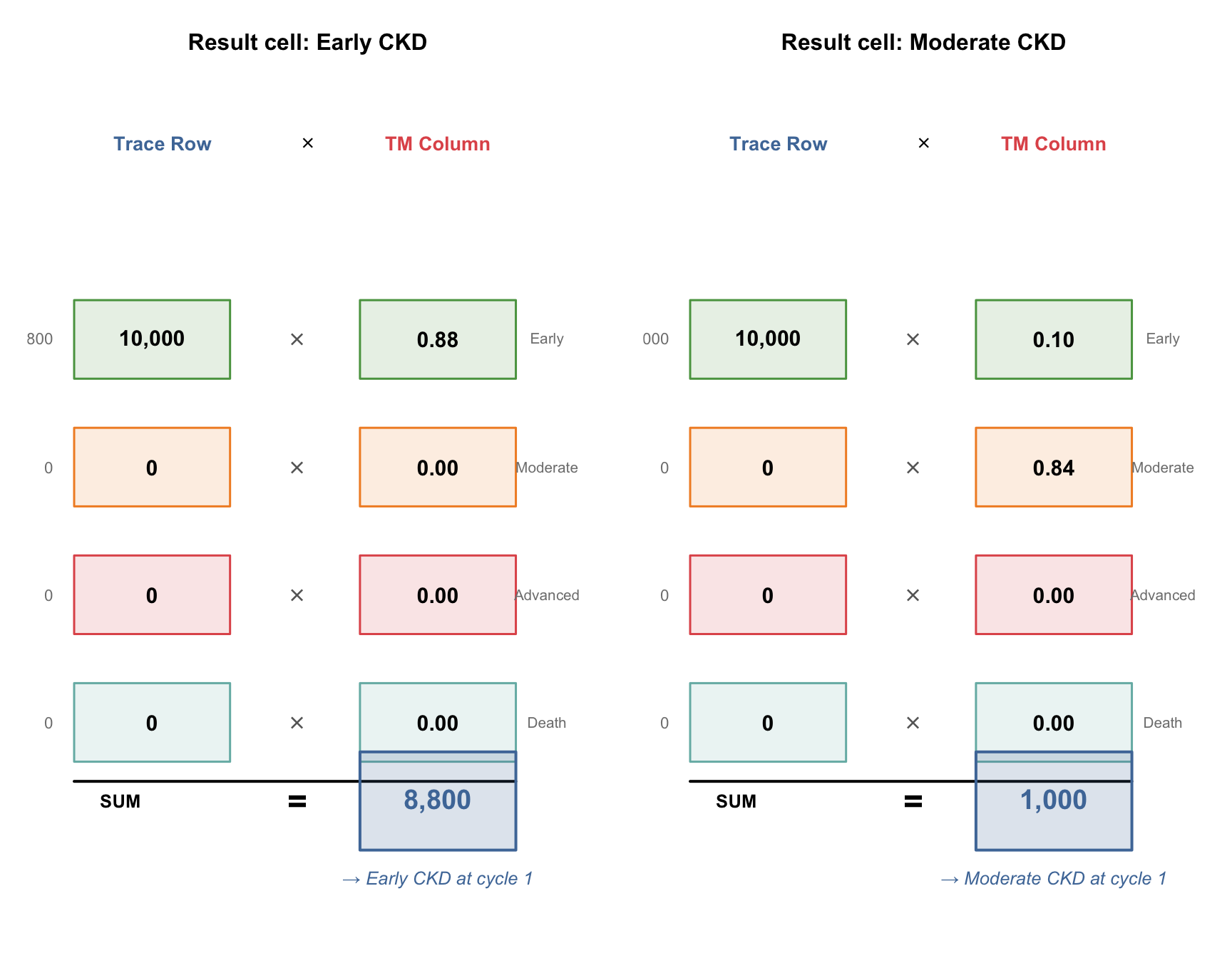
### The "handshake": how one result cell is computed
To compute a single cell in the result, take the **row** from the first matrix and the **column** from the second matrix. Stand them face-to-face, multiply each pair of corresponding elements, and add up all the products. That sum is the cell value.
```{r}
#| label: fig-handshake
#| echo: true
#| fig-cap: "The handshake: row from trace meets column from TM, multiply pairs, sum to get result"
#| fig-height: 7
#| fig-width: 9
# ---------------------------------------------------------------
# HANDSHAKE VISUALISATION
# We show how result[1, "Early CKD"] is computed:
#   trace row meets TM column "Early CKD" face-to-face
# Then repeat for "Moderate CKD" column to show the pattern
# ---------------------------------------------------------------

par(mfrow = c(1, 2), mar = c(1, 1, 3, 1))

# --- Helper function to draw one handshake ---
draw_handshake <- function(row_vals, col_vals, row_labels,
                           result_val, result_label, title_text) {
  plot(NULL, xlim = c(0, 10), ylim = c(-1.5, 6.5), axes = FALSE, ann = FALSE)
  title(main = title_text, cex.main = 1.0, font.main = 2)

  # Column headers
  text(2.2, 6.2, "Trace Row", cex = 0.85, font = 2, col = "#4e79a7")
  text(5.0, 6.2, expression(symbol("\264")), cex = 1.0)
  text(7.5, 6.2, "TM Column", cex = 0.85, font = 2, col = "#e15759")

  # Draw each pair face-to-face
  box_cols <- c("#59a14f", "#f28e2b", "#e15759", "#76b7b2")

  for (i in 1:4) {
    y <- 5.5 - i * 1.3

    # Left box: trace row element
    rect(0.5, y - 0.4, 3.5, y + 0.4,
         col = paste0(box_cols[i], "25"), border = box_cols[i], lwd = 1.5)
    text(2.0, y, format(row_vals[i], big.mark = ","), cex = 0.95, font = 2)

    # Multiplication sign between
    text(4.8, y, expression(symbol("\264")), cex = 1.2, col = "grey40")

    # Right box: TM column element
    rect(6.0, y - 0.4, 9.0, y + 0.4,
         col = paste0(box_cols[i], "25"), border = box_cols[i], lwd = 1.5)
    text(7.5, y, sprintf("%.2f", col_vals[i]), cex = 0.95, font = 2)

    # State label on far right
    text(9.6, y, row_labels[i], cex = 0.65, col = "grey50")

    # Product on far left
    product <- row_vals[i] * col_vals[i]
    text(0.1, y, format(round(product, 1), big.mark = ","),
         cex = 0.7, col = "grey50", adj = 1)
  }

  # Sum line and result
  segments(0.5, -0.3, 9.0, -0.3, lwd = 2, col = "black")
  text(1.0, -0.5, "SUM", cex = 0.8, font = 2, adj = 0)
  text(4.8, -0.5, "=", cex = 1.5, font = 2)

  # Result box
  rect(6.0, -1.0, 9.0, -0.0, col = "#4e79a730", border = "#4e79a7", lwd = 2)
  text(7.5, -0.5, format(round(result_val, 1), big.mark = ","),
       cex = 1.2, font = 2, col = "#4e79a7")
  text(7.5, -1.3, result_label, cex = 0.8, font = 3, col = "#4e79a7")
}

# --- Trace row (cycle 0): all 10,000 in Early CKD ---
trace_row <- c(10000, 0, 0, 0)
labels <- c("Early", "Moderate", "Advanced", "Death")

# Handshake 1: trace row × TM column "Early CKD"
tm_col_early <- tm_standard[, "Early CKD"]
draw_handshake(trace_row, tm_col_early, labels,
               sum(trace_row * tm_col_early),
               "→ Early CKD at cycle 1",
               "Result cell: Early CKD")

# Handshake 2: trace row × TM column "Moderate CKD"
tm_col_mod <- tm_standard[, "Moderate CKD"]
draw_handshake(trace_row, tm_col_mod, labels,
               sum(trace_row * tm_col_mod),
               "→ Moderate CKD at cycle 1",
               "Result cell: Moderate CKD")
```
::: {.callout-tip}
## The Pattern
To fill **every cell** in the result, you repeat this handshake — one for each column of the transition matrix. Since we have 4 states, that's 4 handshakes per cycle. R's `%*%` operator does all 4 at once.
:::
### Cycle 0 → 1: All four results
```{r}
#| label: matmul-demo
#| echo: true
# --- Cycle 0: Starting state ---
trace_0 <- c(10000, 0, 0, 0)
names(trace_0) <- state_names

# R computes all 4 handshakes in one line:
trace_1 <- trace_0 %*% tm_standard
trace_1 <- as.numeric(trace_1)
names(trace_1) <- state_names

# Show the element-by-element computation
handshake_table <- data.frame(
  `Result Cell` = state_names,
  `Dot Product` = c(
    "10000×0.88 + 0×0 + 0×0 + 0×0",
    "10000×0.10 + 0×0.84 + 0×0 + 0×0",
    "10000×0 + 0×0.12 + 0×0.85 + 0×0",
    "10000×0.02 + 0×0.04 + 0×0.15 + 0×1"
  ),
  `= Count` = format(trace_1, big.mark = ","),
  check.names = FALSE
)

kable(handshake_table,
      caption = "Cycle 0 → 1: each result cell is one row × column handshake")
```
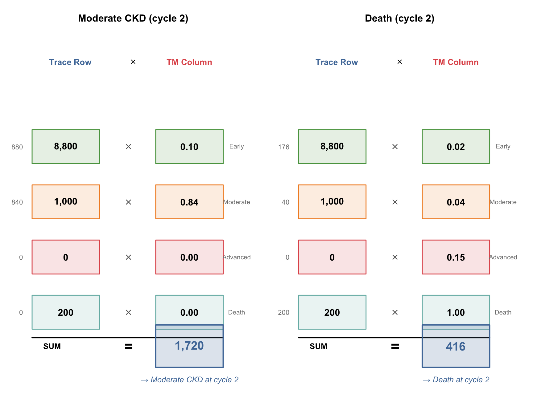
### Cycle 1 → 2: Now it gets interesting
At cycle 1, patients are spread across Early (8,800) and Moderate (1,000) and Death (200). The handshakes now have **multiple non-zero terms**:
```{r}
#| label: fig-handshake-cycle2
#| echo: true
#| fig-cap: "Cycle 1 → 2: with patients in multiple states, the dot products have more non-zero terms"
#| fig-height: 7
#| fig-width: 9
par(mfrow = c(1, 2), mar = c(1, 1, 3, 1))

# Handshake: trace_1 × TM column "Moderate CKD"
tm_col_mod <- tm_standard[, "Moderate CKD"]
draw_handshake(trace_1, tm_col_mod, labels,
               sum(trace_1 * tm_col_mod),
               "→ Moderate CKD at cycle 2",
               "Moderate CKD (cycle 2)")

# Handshake: trace_1 × TM column "Death"
tm_col_death <- tm_standard[, "Death"]
draw_handshake(trace_1, tm_col_death, labels,
               sum(trace_1 * tm_col_death),
               "→ Death at cycle 2",
               "Death (cycle 2)")
```
::: {.callout-note}
## What Changed?
At cycle 0, only one row element was non-zero (10,000 in Early CKD), so each handshake was trivial. By cycle 1, patients occupy multiple states, so the dot products genuinely combine contributions from different states — that's where the model gets its power.
:::
### First 4 cycles — the full trace
```{r}
#| label: matmul-cycles-2-3
#| echo: true
# Cycle 1 → 2
trace_2 <- as.numeric(trace_1 %*% tm_standard)
names(trace_2) <- state_names

# Cycle 2 → 3
trace_3 <- as.numeric(trace_2 %*% tm_standard)
names(trace_3) <- state_names

# Show the first 4 cycles as a table
first_cycles <- data.frame(
  Cycle = 0:3,
  `Early CKD` = c(trace_0[1], trace_1[1], trace_2[1], trace_3[1]),
  `Moderate CKD` = c(trace_0[2], trace_1[2], trace_2[2], trace_3[2]),
  `Advanced/Dialysis` = c(trace_0[3], trace_1[3], trace_2[3], trace_3[3]),
  Death = c(trace_0[4], trace_1[4], trace_2[4], trace_3[4]),
  check.names = FALSE
)

kable(first_cycles, digits = 1,
      caption = "First 4 cycles: watch the cohort flow through states")
```
::: {.callout-note}
## What to Notice
- **Early CKD shrinks** every cycle (patients leave faster than they arrive — no one enters Early CKD)
- **Moderate CKD grows then peaks** — it receives patients from Early but loses them to Advanced and Death
- **Advanced/Dialysis appears at cycle 2** — it takes 2 cycles for the first patients to progress through Early → Moderate → Advanced
- **Death accumulates** — it's absorbing, so it only grows
- **Every row sums to 10,000** — no patients are created or destroyed
:::
## 8. Running the Full Simulation
Now we automate this for all 20 cycles using a loop. The `run_markov()` function also computes costs, QALYs, half-cycle correction, and discounting — we'll explain each of these explicitly in the following sections.
```{r}
#| label: markov-simulation
#| echo: true
# --- Markov Cohort Simulation ---
# Step 1: Create the trace matrix (21 rows × 4 columns)
trace_std <- matrix(0, nrow = n_cycles + 1, ncol = n_states,
                    dimnames = list(paste0("Cycle_", 0:n_cycles), state_names))
trace_std[1, 1] <- n_cohort  # All start in Early CKD

trace_int <- trace_std  # Same starting point for intervention

# Step 2: Run the simulation loop
for (cycle in 1:n_cycles) {
  trace_std[cycle + 1, ] <- trace_std[cycle, ] %*% tm_standard
  trace_int[cycle + 1, ] <- trace_int[cycle, ] %*% tm_intervention
}
```
### The Markov trace table (Standard Care)
This is the raw output of the simulation — the number of patients in each state at each cycle:
```{r}
#| label: trace-table
#| echo: true
# Show first 6 and last 3 cycles
trace_display <- as.data.frame(round(trace_std, 1))
trace_display$Cycle <- 0:n_cycles
trace_display$Total <- rowSums(trace_std)
trace_display <- trace_display[, c("Cycle", state_names, "Total")]

# Show selected rows
rows_to_show <- c(1:6, 11, 16, 21)  # cycles 0-5, 10, 15, 20
kable(trace_display[rows_to_show, ], digits = 1, row.names = FALSE,
      caption = "Markov trace (Standard Care): patient counts per state")
```
::: {.callout-note}
## Verify: Total column
Every row sums to exactly 10,000 — the cohort is closed (no patients enter or leave the model, they just move between states). This is a useful sanity check.
:::
## 9. Half-Cycle Correction
The simulation tells us the state at the **start** of each cycle (cycle 0, 1, 2, ...). But patients transition *during* the cycle, not instantaneously at the start or end. Half-cycle correction approximates the **average** occupancy during each cycle by averaging the start and end counts:
$$\text{HCC}_t = \frac{\text{trace}_{t-1} + \text{trace}_t}{2}$$
```{r}
#| label: half-cycle
#| echo: true
# Half-cycle corrected trace: average start and end of each cycle
trace_hcc_std <- (trace_std[1:n_cycles, ] + trace_std[2:(n_cycles + 1), ]) / 2
trace_hcc_int <- (trace_int[1:n_cycles, ] + trace_int[2:(n_cycles + 1), ]) / 2

# Show the difference for cycle 1
kable(data.frame(
  Measure = c("Start of cycle 1 (trace row 1)",
              "End of cycle 1 (trace row 2)",
              "Half-cycle corrected average"),
  `Early CKD` = c(trace_std[1, 1], trace_std[2, 1],
                   trace_hcc_std[1, 1]),
  `Moderate CKD` = c(trace_std[1, 2], trace_std[2, 2],
                      trace_hcc_std[1, 2]),
  `Adv/Dialysis` = c(trace_std[1, 3], trace_std[2, 3],
                      trace_hcc_std[1, 3]),
  Death = c(trace_std[1, 4], trace_std[2, 4],
            trace_hcc_std[1, 4]),
  check.names = FALSE
), digits = 1, caption = "Half-cycle correction for cycle 1: averaging start and end")
```
::: {.callout-tip}
## Why Does This Matter?
Without half-cycle correction, we'd either assume all transitions happen at the start of the year (overestimating time in new states) or at the end (underestimating). The average is a better approximation of reality. The effect is small per cycle but accumulates over 20 years. This is a standard technical requirement in published HTA models.
:::
## 10. Discounting
Society values benefits today more than benefits in the future — a concept called **time preference**. In HTA, we account for this by **discounting** future costs and QALYs. India's standard discount rate is **3% per year**.
The discount factor for cycle $t$ (starting from 0) is:
$$d_t = \frac{1}{(1 + r)^t}$$
where $r$ = 0.03. This means ₹1,00,000 in year 10 is worth only ₹74,409 in today's terms.
```{r}
#| label: discounting
#| echo: true
# Discount factors for each cycle
discount_factors <- 1 / (1 + discount_rate)^(0:(n_cycles - 1))

# Show the first few
kable(data.frame(
  Cycle = 1:10,
  `Discount Factor` = round(discount_factors[1:10], 4),
  `₹1,00,000 worth today` = paste0("₹", format(round(100000 * discount_factors[1:10]), big.mark = ",")),
  check.names = FALSE
), caption = "Discount factors: ₹1,00,000 in future years expressed in today's value")
```
## 11. Costs, QALYs, and ICER
Now we combine the half-cycle corrected trace with costs, utilities, and discount factors to compute total costs and QALYs for each strategy:
```{r}
#| label: cost-qaly-calculation
#| echo: true
# Cost and utility vectors
costs_standard     <- c(cost_early, cost_moderate, cost_advanced, cost_death)
costs_intervention <- c(cost_early + cost_ace_annual,   # ACE-inhibitor added
                        cost_moderate + cost_ace_annual,
                        cost_advanced,   # ACE-inhibitor usually stopped in advanced CKD
                        cost_death)
utilities <- c(utility_early, utility_moderate, utility_advanced, utility_death)

# Cycle costs = HCC trace × cost vector (matrix multiplication)
cycle_costs_std <- trace_hcc_std %*% costs_standard
cycle_costs_int <- trace_hcc_int %*% costs_intervention

# Cycle QALYs = HCC trace × utility vector
cycle_qalys_std <- trace_hcc_std %*% utilities
cycle_qalys_int <- trace_hcc_int %*% utilities

# Apply discounting
disc_costs_std <- cycle_costs_std * discount_factors
disc_costs_int <- cycle_costs_int * discount_factors
disc_qalys_std <- cycle_qalys_std * discount_factors
disc_qalys_int <- cycle_qalys_int * discount_factors

# Total across all cycles
total_cost_std <- sum(disc_costs_std)
total_cost_int <- sum(disc_costs_int) + n_cohort * cost_screening  # add one-time screening
total_qaly_std <- sum(disc_qalys_std)
total_qaly_int <- sum(disc_qalys_int)

# ICER
inc_cost <- total_cost_int - total_cost_std
inc_qaly <- total_qaly_int - total_qaly_std
icer <- inc_cost / inc_qaly
```
### Results summary
```{r}
#| label: results-table
#| echo: true
results_summary <- data.frame(
  Strategy = c("Standard Care", "Screening + ACE-inhibitor", "Incremental"),
  `Total Cost (₹)` = c(
    format(round(total_cost_std), big.mark = ","),
    format(round(total_cost_int), big.mark = ","),
    format(round(inc_cost), big.mark = ",")
  ),
  `Total QALYs` = c(
    round(total_qaly_std, 1),
    round(total_qaly_int, 1),
    round(inc_qaly, 1)
  ),
  `Per Patient Cost` = c(
    paste0("₹", format(round(total_cost_std / n_cohort), big.mark = ",")),
    paste0("₹", format(round(total_cost_int / n_cohort), big.mark = ",")),
    paste0("₹", format(round(inc_cost / n_cohort), big.mark = ","))
  ),
  `Per Patient QALYs` = c(
    round(total_qaly_std / n_cohort, 4),
    round(total_qaly_int / n_cohort, 4),
    round(inc_qaly / n_cohort, 4)
  ),
  check.names = FALSE
)

kable(results_summary, align = "lrrrr",
      caption = "Cost-effectiveness results (20-year horizon, 3% discounting)")
```
```{r}
#| label: icer-interpretation
#| echo: true
# -------------------------------------------------------
# ICER interpretation — handle the negative ICER carefully
# -------------------------------------------------------
# A negative ICER can mean TWO very different things:
#   1. inc_cost < 0 AND inc_qaly > 0 → DOMINANT (saves money, gains health)
#   2. inc_cost > 0 AND inc_qaly < 0 → DOMINATED (costs more, loses health)
# Both give a negative ratio, but the conclusions are opposite!
# This is why many HTA guidelines recommend AGAINST relying on the ICER alone
# and instead use Net Monetary Benefit (NMB).

icer_formatted <- format(round(icer), big.mark = ",")

interpretation <- if (inc_cost < 0 & inc_qaly > 0) {
  "DOMINANT — the intervention saves costs AND improves health"
} else if (inc_cost > 0 & inc_qaly < 0) {
  "DOMINATED — the intervention costs more AND worsens health"
} else if (inc_cost > 0 & inc_qaly > 0) {
  # Standard ICER quadrant (NE): compare to WTP
  if (icer < wtp_india) {
    paste0("Cost-effective (ICER < WTP of ₹", format(wtp_india, big.mark = ","), ")")
  } else {
    "NOT cost-effective at conventional thresholds"
  }
} else {
  # inc_cost < 0, inc_qaly < 0 (SW quadrant): intervention cheaper but worse
  paste0("Trade-off: saves money but loses QALYs (ICER = ₹", icer_formatted, ")")
}

kable(data.frame(
  Metric = c("Incremental Cost", "Incremental QALYs", "ICER",
             "WTP Threshold (1× GDP/capita)", "Conclusion"),
  Value = c(paste0("₹", format(round(inc_cost / n_cohort), big.mark = ","), " per patient"),
            paste0(round(inc_qaly / n_cohort, 4), " per patient"),
            paste0("₹", icer_formatted, " per QALY gained"),
            paste0("₹", format(wtp_india, big.mark = ",")),
            interpretation),
  check.names = FALSE
), caption = "Cost-effectiveness conclusion")
```
::: {.callout-warning}
## Why a Negative ICER Is Ambiguous
The ICER is a *ratio*: ΔCost ÷ ΔQALYs. A negative ratio appears when the numerator and denominator have opposite signs — but that happens in **two** situations:
| | ΔQALYs > 0 (better) | ΔQALYs < 0 (worse) |
|---|---|---|
| **ΔCost > 0 (costlier)** | NE quadrant: standard ICER | SE quadrant: **DOMINATED** |
| **ΔCost < 0 (cheaper)** | NW quadrant: **DOMINANT** | SW quadrant: trade-off |
Both DOMINANT and DOMINATED produce a negative ICER, but the conclusions are opposite. **Always check the signs of ΔCost and ΔQALYs separately** — never rely on the ICER sign alone. This is exactly why the Net Monetary Benefit (NMB) was developed: it gives an unambiguous single number.
:::
### Net Monetary Benefit (NMB)
The NMB converts QALYs into monetary terms using the WTP threshold, then subtracts costs. A positive incremental NMB means the intervention is cost-effective — no sign ambiguity.
$$\text{NMB} = (\text{WTP} \times \text{QALYs}) - \text{Cost}$$
$$\Delta\text{NMB} = \text{NMB}_{\text{intervention}} - \text{NMB}_{\text{standard}} = (\text{WTP} \times \Delta\text{QALYs}) - \Delta\text{Cost}$$
If ΔNMB > 0 → cost-effective. If ΔNMB < 0 → not cost-effective. **No quadrant confusion.**
```{r}
#| label: nmb-calculation
#| echo: true
# Net Monetary Benefit per patient
nmb_std <- (wtp_india * total_qaly_std / n_cohort) - (total_cost_std / n_cohort)
nmb_int <- (wtp_india * total_qaly_int / n_cohort) - (total_cost_int / n_cohort)
inc_nmb <- nmb_int - nmb_std

# Equivalently: WTP × ΔQALYs − ΔCost
inc_nmb_check <- wtp_india * (inc_qaly / n_cohort) - (inc_cost / n_cohort)

kable(data.frame(
  Metric = c("NMB Standard Care", "NMB Intervention",
             "Incremental NMB (ΔNMB)", "Decision"),
  Value = c(
    paste0("₹", format(round(nmb_std), big.mark = ",")),
    paste0("₹", format(round(nmb_int), big.mark = ",")),
    paste0("₹", format(round(inc_nmb), big.mark = ",")),
    if (inc_nmb > 0) "ADOPT — positive ΔNMB" else "REJECT — negative ΔNMB"
  ),
  check.names = FALSE
), caption = paste0("Net Monetary Benefit analysis (WTP = ₹", format(wtp_india, big.mark = ","), "/QALY)"))
```
::: {.callout-tip}
## When to Use NMB vs ICER
The **ICER** is great for communication — "the intervention costs ₹X per QALY gained" is intuitive. But for **decision-making**, NMB is safer: it's always unambiguous, and it's essential for probabilistic sensitivity analysis (PSA) where you need to compare across thousands of iterations — you can't average ICERs, but you can average NMBs.
**Rule of thumb:** Report the ICER in your results, but use NMB for the actual decision and for sensitivity analysis.
:::
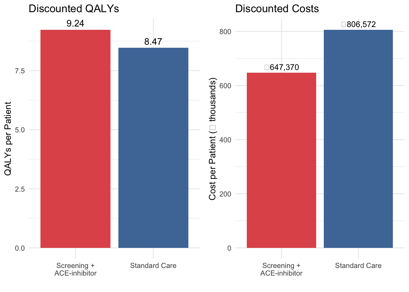
```{r}
#| label: fig-qaly-breakdown
#| echo: true
#| fig-cap: "Discounted costs and QALYs per patient by strategy"
library(gridExtra)

qaly_data <- data.frame(
  Strategy = c("Standard Care", "Screening +\nACE-inhibitor"),
  Total_QALY = c(total_qaly_std / n_cohort, total_qaly_int / n_cohort),
  Total_Cost = c(total_cost_std / n_cohort, total_cost_int / n_cohort)
)

p1 <- ggplot(qaly_data, aes(x = Strategy, y = Total_QALY, fill = Strategy)) +
  geom_col(show.legend = FALSE) +
  geom_text(aes(label = round(Total_QALY, 2)), vjust = -0.5, size = 4) +
  scale_fill_manual(values = c("#e15759", "#4e79a7")) +
  labs(x = "", y = "QALYs per Patient", title = "Discounted QALYs") +
  theme_minimal()

p2 <- ggplot(qaly_data, aes(x = Strategy, y = Total_Cost / 1000, fill = Strategy)) +
  geom_col(show.legend = FALSE) +
  geom_text(aes(label = paste0("₹", format(round(Total_Cost), big.mark = ","))),
            vjust = -0.5, size = 3.5) +
  scale_fill_manual(values = c("#e15759", "#4e79a7")) +
  labs(x = "", y = "Cost per Patient (₹ thousands)", title = "Discounted Costs") +
  theme_minimal()

grid.arrange(p1, p2, ncol = 2)
```
## 12. Visualising the Markov Trace
```{r}
#| label: fig-markov-trace
#| echo: true
#| fig-cap: "Markov trace: cohort distribution over 20 years"
trace_df_std <- as.data.frame(trace_std / n_cohort)
trace_df_std$Cycle <- 0:n_cycles
trace_df_std$Strategy <- "Standard Care"
trace_df_int <- as.data.frame(trace_int / n_cohort)
trace_df_int$Cycle <- 0:n_cycles
trace_df_int$Strategy <- "Screening + ACE-inhibitor"
trace_combined <- rbind(trace_df_std, trace_df_int)
trace_long <- pivot_longer(trace_combined,
cols = all_of(state_names),
names_to = "State",
values_to = "Proportion")
trace_long$State <- factor(trace_long$State, levels = state_names)
ggplot(trace_long, aes(x = Cycle, y = Proportion, fill = State)) +
geom_area(alpha = 0.8) +
facet_wrap(~Strategy) +
scale_fill_manual(values = c("Early CKD" = "#59a14f",
"Moderate CKD" = "#f28e2b",
"Advanced/Dialysis" = "#e15759",
"Death" = "#76b7b2")) +
labs(
x = "Year", y = "Proportion of Cohort",
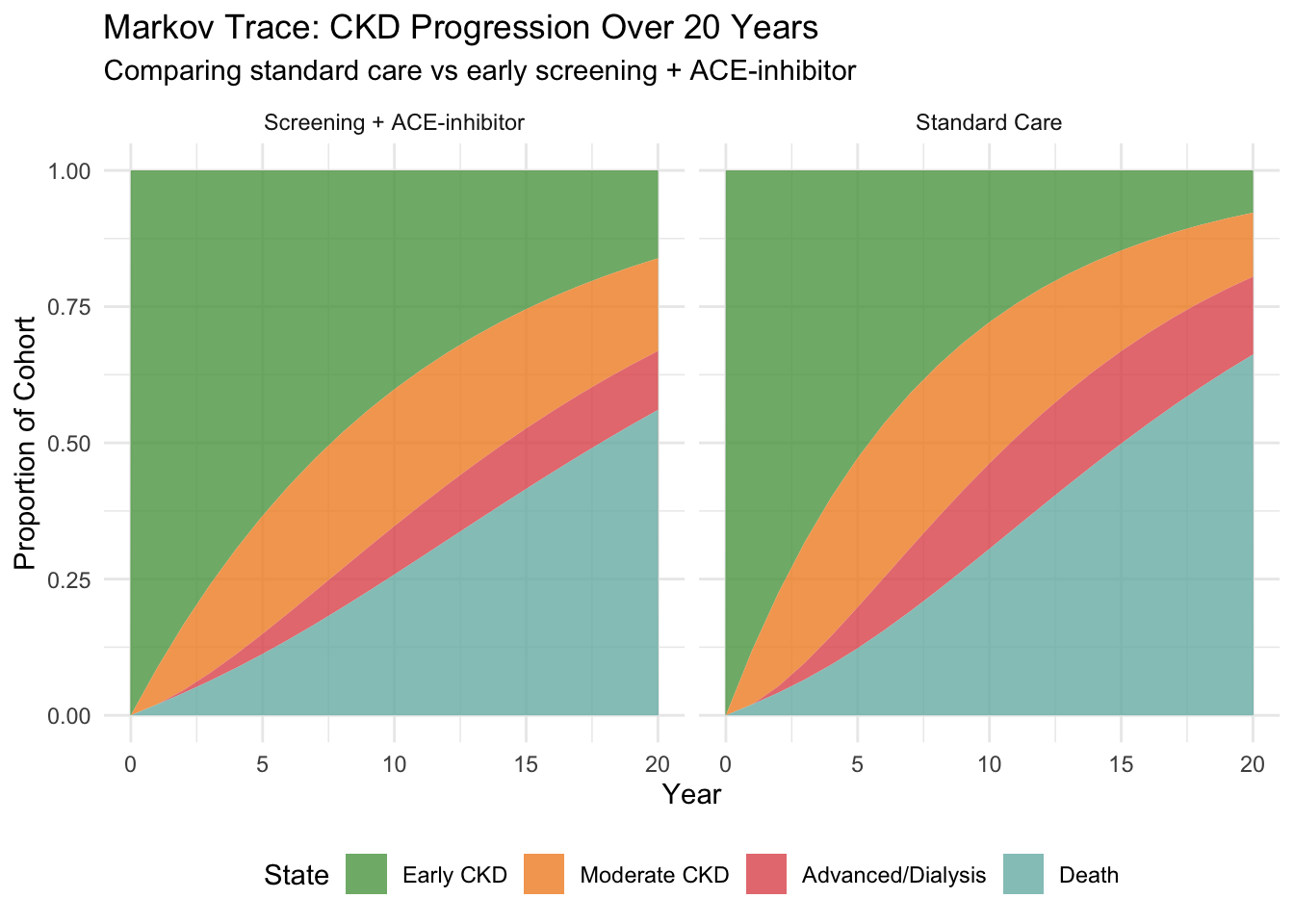
title = "Markov Trace: CKD Progression Over 20 Years",
subtitle = "Comparing standard care vs early screening + ACE-inhibitor"
) +
theme_minimal() +
theme(legend.position = "bottom")
```
::: {.callout-tip}
## Reading the Markov Trace
The green area (Early CKD) shrinks over time as patients progress. The intervention keeps more patients in green for longer — that's the visual signature of a drug that slows progression. The red area (Advanced/Dialysis) grows more slowly in the intervention arm. Since dialysis costs ₹3,50,000/year, this delay translates directly into cost savings.
:::
## 13. Patients Reaching Dialysis
```{r}
#| label: fig-dialysis
#| echo: true
#| fig-cap: "Proportion of cohort in Advanced CKD/Dialysis over time"
dialysis_data <- data.frame(
Year = rep(0:n_cycles, 2),
Proportion = c(trace_std[, "Advanced/Dialysis"] / n_cohort,
trace_int[, "Advanced/Dialysis"] / n_cohort),
Strategy = rep(c("Standard Care", "Screening + ACE-inhibitor"), each = n_cycles + 1)
)
ggplot(dialysis_data, aes(x = Year, y = Proportion * 100, colour = Strategy)) +
geom_line(linewidth = 1.2) +
labs(x = "Year", y = "% of Cohort on Dialysis",
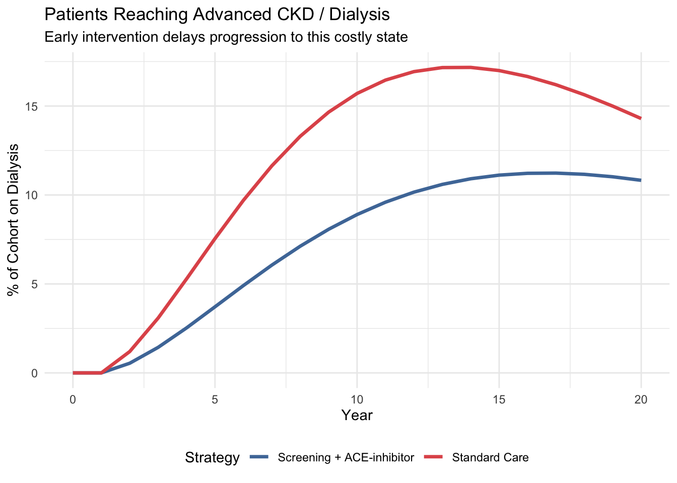
title = "Patients Reaching Advanced CKD / Dialysis",
subtitle = "Early intervention delays progression to this costly state") +
scale_colour_manual(values = c("Standard Care" = "#e15759",
"Screening + ACE-inhibitor" = "#4e79a7")) +
theme_minimal() +
theme(legend.position = "bottom")
```
## 14. Cost Accumulation Over Time
```{r}
#| label: fig-cumcost
#| echo: true
#| fig-cap: "Cumulative discounted costs per patient over 20 years"
cumcost_std <- cumsum(disc_costs_std) / n_cohort
cumcost_int <- cumsum(disc_costs_int) / n_cohort + cost_screening
cost_over_time <- data.frame(
Year = rep(1:n_cycles, 2),
Cumulative_Cost = c(cumcost_std, cumcost_int),
Strategy = rep(c("Standard Care", "Screening + ACE-inhibitor"), each = n_cycles)
)
ggplot(cost_over_time, aes(x = Year, y = Cumulative_Cost / 1000, colour = Strategy)) +
geom_line(linewidth = 1.2) +
labs(x = "Year", y = "Cumulative Cost per Patient (₹ thousands)",
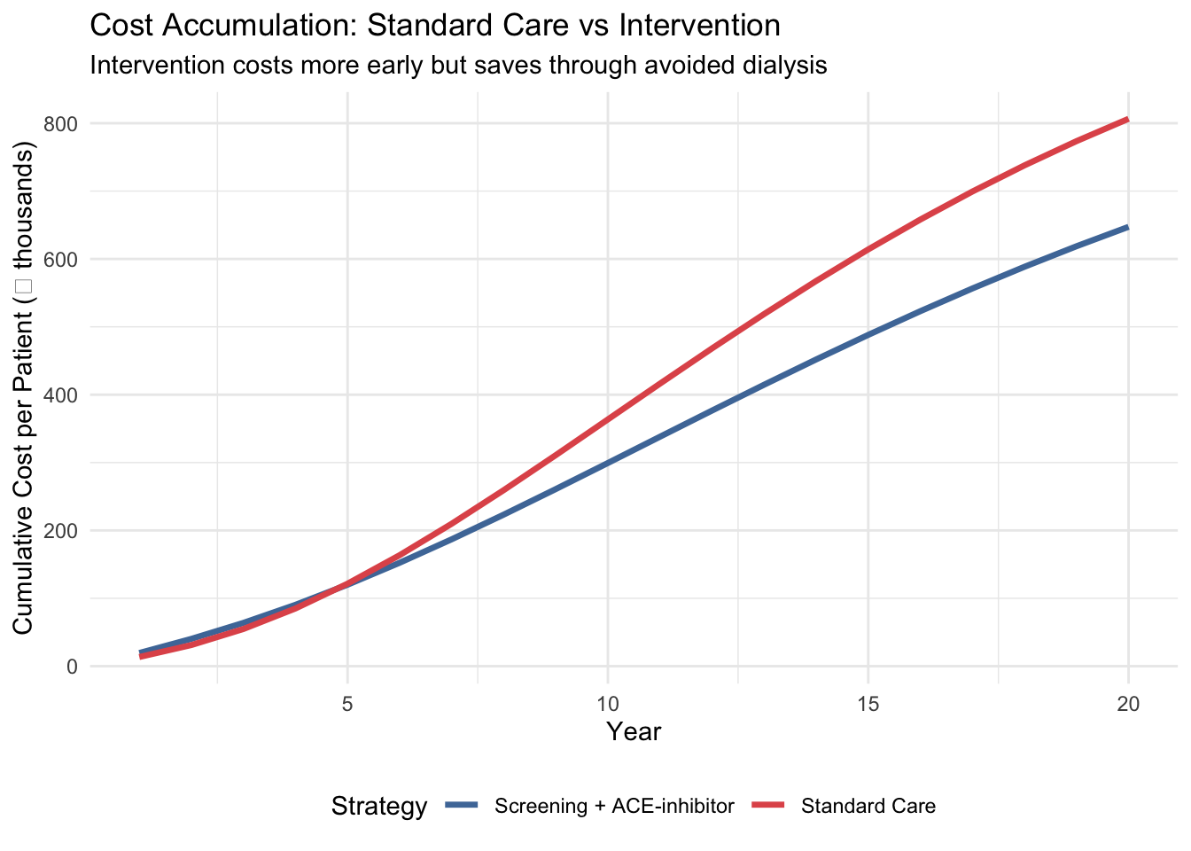
title = "Cost Accumulation: Standard Care vs Intervention",
subtitle = "Intervention costs more early but saves through avoided dialysis") +
scale_colour_manual(values = c("Standard Care" = "#e15759",
"Screening + ACE-inhibitor" = "#4e79a7")) +
theme_minimal() +
theme(legend.position = "bottom")
```
## 15. Quick Sensitivity Check
Before declaring a result "cost-effective", we should ask: **how sensitive is the ICER to our assumptions?** Here we vary the two most influential parameters — dialysis cost and treatment efficacy — one at a time.
::: {.callout-note}
## Preview Only
This is a brief demonstration. Session 6 covers Probabilistic Sensitivity Analysis (PSA) in full depth, including simultaneous variation of all uncertain parameters.
:::
```{r}
#| label: one-way-sa
#| echo: true
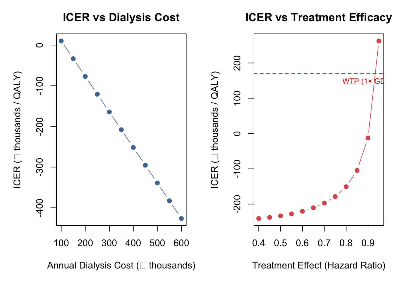
#| fig-cap: "One-way sensitivity analysis: ICER vs dialysis cost and treatment effect"
# Helper function to run one arm (avoids repeating the full loop)
run_arm <- function(tm, cost_vec, n_cohort, n_cycles, utilities, discount_rate) {
  trace <- matrix(0, nrow = n_cycles + 1, ncol = 4)
  trace[1, 1] <- n_cohort
  for (c in 1:n_cycles) trace[c + 1, ] <- trace[c, ] %*% tm
  hcc <- (trace[1:n_cycles, ] + trace[2:(n_cycles + 1), ]) / 2
  df <- 1 / (1 + discount_rate)^(0:(n_cycles - 1))
  list(cost = sum((hcc %*% cost_vec) * df),
       qaly = sum((hcc %*% utilities) * df))
}

# --- One-Way SA: Dialysis Cost ---
dialysis_range <- seq(100000, 600000, by = 50000)
icer_by_dialysis <- numeric(length(dialysis_range))

for (i in seq_along(dialysis_range)) {
  cs <- c(cost_early, cost_moderate, dialysis_range[i], 0)
  ci <- c(cost_early + cost_ace_annual, cost_moderate + cost_ace_annual, dialysis_range[i], 0)
  rs <- run_arm(tm_standard, cs, n_cohort, n_cycles, utilities, discount_rate)
  ri <- run_arm(tm_intervention, ci, n_cohort, n_cycles, utilities, discount_rate)
  ri$cost <- ri$cost + n_cohort * cost_screening
  icer_by_dialysis[i] <- (ri$cost - rs$cost) / (ri$qaly - rs$qaly)
}

# --- One-Way SA: Treatment Effect (HR) ---
hr_range <- seq(0.40, 0.95, by = 0.05)
icer_by_hr <- numeric(length(hr_range))

for (i in seq_along(hr_range)) {
  p12i <- 1 - (1 - p_12_standard)^hr_range[i]
  p23i <- 1 - (1 - p_23_standard)^hr_range[i]
  tm_sa <- tm_standard
  tm_sa[1, 2] <- p12i; tm_sa[1, 1] <- 1 - p12i - p_1d_standard
  tm_sa[2, 3] <- p23i; tm_sa[2, 2] <- 1 - p23i - p_2d_standard
  rs <- run_arm(tm_standard, costs_standard, n_cohort, n_cycles, utilities, discount_rate)
  ri <- run_arm(tm_sa, costs_intervention, n_cohort, n_cycles, utilities, discount_rate)
  ri$cost <- ri$cost + n_cohort * cost_screening
  icer_by_hr[i] <- (ri$cost - rs$cost) / (ri$qaly - rs$qaly)
}

# --- Plot Both ---
par(mfrow = c(1, 2), mar = c(5, 5, 3, 1))

plot(dialysis_range / 1000, icer_by_dialysis / 1000, type = "b", pch = 19,
     col = "#4e79a7", xlab = "Annual Dialysis Cost (₹ thousands)",
     ylab = "ICER (₹ thousands / QALY)", main = "ICER vs Dialysis Cost")
abline(h = wtp_india / 1000, col = "red", lty = 2)
text(max(dialysis_range) / 1000, wtp_india / 1000, "WTP (1× GDP/capita)",
     pos = 1, col = "red", cex = 0.8)

plot(hr_range, icer_by_hr / 1000, type = "b", pch = 19,
     col = "#e15759", xlab = "Treatment Effect (Hazard Ratio)",
     ylab = "ICER (₹ thousands / QALY)", main = "ICER vs Treatment Efficacy")
abline(h = wtp_india / 1000, col = "red", lty = 2)
text(max(hr_range), wtp_india / 1000, "WTP (1× GDP/capita)",
     pos = 1, col = "red", cex = 0.8)
```
::: {.callout-tip}
## What This Tells Us
The ICER is most sensitive to dialysis cost — the more expensive dialysis is, the more money the intervention saves by keeping patients out of that state. The treatment effect also matters: as the hazard ratio approaches 1.0 (no effect), the ICER rises steeply. Notice that all ICERs here remain negative (dominant) — in PSA, where ICERs can flip between quadrants across iterations, we'd use NMB instead.
:::
## 16. Cross-Validation Checkpoint
A critical step in any HTA model is **cross-validation** — verifying your R results against an independent implementation. We provide an Excel companion model (`CKD-Markov-Model.xlsx`) for this purpose.
```{r}
#| label: cross-validation
#| echo: true
# Cross-validation reference table
xval <- data.frame(
  Metric = c("Standard: Cost/patient", "Standard: QALYs/patient",
             "Intervention: Cost/patient", "Intervention: QALYs/patient",
             "Incremental cost/patient", "Incremental QALYs/patient", "ICER"),
  `R Value` = c(
    paste0("₹", format(round(total_cost_std / n_cohort), big.mark = ",")),
    round(total_qaly_std / n_cohort, 4),
    paste0("₹", format(round(total_cost_int / n_cohort), big.mark = ",")),
    round(total_qaly_int / n_cohort, 4),
    paste0("₹", format(round(inc_cost / n_cohort), big.mark = ",")),
    round(inc_qaly / n_cohort, 4),
    paste0("₹", format(round(icer), big.mark = ","))
  ),
  `Excel Value` = rep("← check", 7),
  Match = rep("?", 7),
  check.names = FALSE
)

kable(xval, caption = "Cross-validation checklist: fill in Excel values and verify match")
```
::: {.callout-important}
## Why Cross-Validate?
If your R ICER and your Excel ICER differ by more than ₹1–2 (rounding), something is wrong. Common sources of mismatch: forgetting half-cycle correction in Excel, discount factor indexing off by one cycle, or computing the "stay" probability as `1 - p_progression` instead of `1 - p_progression - p_death`.
:::
## 17. What You Just Did
You built a complete **Markov cohort model** — the most common model type in HTA worldwide — step by step:
1. **Health states** — the distinct conditions patients can be in
2. **HR → probability conversion** — translating clinical trial evidence into model inputs
3. **Transition matrix** — scaffold, populate, verify row sums
4. **Matrix multiplication** — the one-line simulation engine
5. **Markov trace** — raw counts table + area chart
6. **Half-cycle correction** — averaging cycle start/end for accuracy
7. **Discounting** — applying time preference at 3% per year
8. **ICER** — incremental cost per QALY gained, with careful sign handling
9. **NMB** — Net Monetary Benefit for unambiguous decision-making
10. **One-way sensitivity analysis** — testing robustness to key assumptions
In R, the core simulation is a single line: `trace[cycle + 1, ] <- trace[cycle, ] %*% tm` — matrix multiplication handles all transitions at once.
→ **Next:** Open `ckd-exercise.qmd` to explore how changing parameters affects the model, then try the **[Session 5 Bonus: heemod Package](ckd-markov-heemod.qmd)** to see the same model built with a dedicated Markov modelling package.
## Key References
- Go AS et al. (2004). Chronic kidney disease and the risks of death and hospitalisation. *NEJM*.
- Singh AK et al. (2013). Epidemiology and risk factors of CKD in India — SEEK study. *BMC Nephrology*.
- Rajapurkar MM et al. (2012). CKD in India: a clarion call for change. *Lancet*.
- ACC/AHA (2024). Risk of initiating ACEi/ARBs in advanced CKD.
- Inside CKD Investigators (2024). Economic burden of CKD at the patient level. *Lancet eClinicalMedicine*.
- Hou FF et al. (2006). ACE inhibitor in progressive renal disease. *NEJM*.
- Indian CKD Registry. BMC Nephrology 2012.