---
title: "Session 3 (Bonus): GDM Screening Using the `rdecision` Package"
subtitle: "Same diagnostic model, built with a dedicated HTA decision tree package"
format:
html:
toc: true
code-fold: show
code-tools: true
---
## Why This Bonus Page Exists
In Session 3, we built the GDM diagnostic decision tree **from scratch** — manually counting true positives, false negatives, computing costs and QALYs for each pathway. That transparency is essential for understanding what a diagnostic model does.
Now we rebuild the **same model** using [`rdecision`](https://cran.r-project.org/package=rdecision), a dedicated R package for decision-analytic modelling. The goal:
1. **Results match** — same parameters, same ICERs, same NMB ranking
2. **Code is shorter** — node-based tree construction replaces manual pathway arithmetic
3. **PSA is built in** — attach distributions and run Monte Carlo with one method call
4. **Pattern recognition** — you'll see the same package used in Session 4 for the DES vs BMS tree
::: {.callout-note}
## Install first
```r
install.packages("rdecision")
```
:::
## 1. Parameters — Identical to Session 3
We use the **exact same inputs** so we can cross-validate.
```{r}
#| label: parameters
#| echo: true
library(rdecision)
library(knitr)

# --- Prevalence ---
prev_gdm <- 0.12
n_cohort <- 10000

# --- Test Accuracy ---
sens_ogtt <- 0.90
spec_ogtt <- 0.85

# --- Costs (₹) ---
cost_ogtt <- 250
cost_risk_assessment <- 50
cost_gdm_treatment <- 8000
cost_adverse <- 45000
cost_no_adverse <- 5000

# --- Probabilities ---
p_adverse_gdm_treated   <- 0.10
p_adverse_gdm_untreated <- 0.35
p_adverse_no_gdm        <- 0.05

# --- Utilities ---
utility_adverse    <- 0.65
utility_no_adverse <- 0.90
utility_gdm_treated <- 0.82

# --- Risk-based screening ---
prop_high_risk <- 0.60
prev_gdm_high_risk <- 0.18
prev_gdm_low_risk  <- 0.03
detection_rate_clinical <- 0.25

# --- WTP ---
wtp_india <- 170000
```
## 2. Building the Universal Screening Tree
In `rdecision`, we build trees from three types of objects: `DecisionNode` (where we choose), `ChanceNode` (where nature decides), and `LeafNode` (terminal outcomes with cost and utility). Edges connect them via `Action` (from decisions) and `Reaction` (from chance nodes).
For the universal screening strategy, the tree structure is:
**Screen → GDM+ (12%) / GDM- (88%) → Test result → Adverse / No adverse**
```{r}
#| label: universal-tree
#| echo: true
# ============================================================
# UNIVERSAL SCREENING TREE
# ============================================================

# --- Leaf nodes: terminal outcomes ---
# True Positive path (GDM detected, treated)
leaf_tp_adverse <- LeafNode$new("TP Adverse",
  utility = utility_adverse,
  interval = as.difftime(365.25, units = "days"))
leaf_tp_well <- LeafNode$new("TP Well",
  utility = utility_gdm_treated,
  interval = as.difftime(365.25, units = "days"))

# False Negative path (GDM missed, untreated)
leaf_fn_adverse <- LeafNode$new("FN Adverse",
  utility = utility_adverse,
  interval = as.difftime(365.25, units = "days"))
leaf_fn_well <- LeafNode$new("FN Well",
  utility = utility_no_adverse,
  interval = as.difftime(365.25, units = "days"))

# False Positive path (no GDM, treated unnecessarily)
leaf_fp_adverse <- LeafNode$new("FP Adverse",
  utility = utility_adverse,
  interval = as.difftime(365.25, units = "days"))
leaf_fp_well <- LeafNode$new("FP Well",
  utility = utility_gdm_treated,
  interval = as.difftime(365.25, units = "days"))

# True Negative path (no GDM, correctly cleared)
leaf_tn_adverse <- LeafNode$new("TN Adverse",
  utility = utility_adverse,
  interval = as.difftime(365.25, units = "days"))
leaf_tn_well <- LeafNode$new("TN Well",
  utility = utility_no_adverse,
  interval = as.difftime(365.25, units = "days"))

# --- Chance nodes: adverse outcomes ---
cn_tp_outcome <- ChanceNode$new("TP Outcome")
cn_fn_outcome <- ChanceNode$new("FN Outcome")
cn_fp_outcome <- ChanceNode$new("FP Outcome")
cn_tn_outcome <- ChanceNode$new("TN Outcome")

# --- Chance nodes: test results ---
cn_gdm_pos <- ChanceNode$new("GDM+ Test")
cn_gdm_neg <- ChanceNode$new("GDM- Test")

# --- Chance node: disease status ---
cn_disease <- ChanceNode$new("Disease Status")

# --- Reactions (edges from chance nodes) ---
# Disease status
r_gdm <- Reaction$new(cn_disease, cn_gdm_pos, p = prev_gdm, label = "GDM+")
r_no_gdm <- Reaction$new(cn_disease, cn_gdm_neg, p = 1 - prev_gdm, label = "GDM-")

# Test results for GDM+ women
r_tp <- Reaction$new(cn_gdm_pos, cn_tp_outcome, p = sens_ogtt,
                      cost = cost_gdm_treatment, label = "Test+ (TP)")
r_fn <- Reaction$new(cn_gdm_pos, cn_fn_outcome, p = 1 - sens_ogtt,
                      label = "Test- (FN)")

# Test results for GDM- women
r_fp <- Reaction$new(cn_gdm_neg, cn_fp_outcome, p = 1 - spec_ogtt,
                      cost = cost_gdm_treatment, label = "Test+ (FP)")
r_tn <- Reaction$new(cn_gdm_neg, cn_tn_outcome, p = spec_ogtt,
                      label = "Test- (TN)")

# Adverse outcomes by pathway
r_tp_adv <- Reaction$new(cn_tp_outcome, leaf_tp_adverse, p = p_adverse_gdm_treated,
                          cost = cost_adverse, label = "Adverse")
r_tp_well <- Reaction$new(cn_tp_outcome, leaf_tp_well, p = 1 - p_adverse_gdm_treated,
                           cost = cost_no_adverse, label = "Well")

r_fn_adv <- Reaction$new(cn_fn_outcome, leaf_fn_adverse, p = p_adverse_gdm_untreated,
                          cost = cost_adverse, label = "Adverse")
r_fn_well <- Reaction$new(cn_fn_outcome, leaf_fn_well, p = 1 - p_adverse_gdm_untreated,
                           cost = cost_no_adverse, label = "Well")

r_fp_adv <- Reaction$new(cn_fp_outcome, leaf_fp_adverse, p = p_adverse_no_gdm,
                          cost = cost_adverse, label = "Adverse")
r_fp_well <- Reaction$new(cn_fp_outcome, leaf_fp_well, p = 1 - p_adverse_no_gdm,
                           cost = cost_no_adverse, label = "Well")

r_tn_adv <- Reaction$new(cn_tn_outcome, leaf_tn_adverse, p = p_adverse_no_gdm,
                          cost = cost_adverse, label = "Adverse")
r_tn_well <- Reaction$new(cn_tn_outcome, leaf_tn_well, p = 1 - p_adverse_no_gdm,
                           cost = cost_no_adverse, label = "Well")

# --- Decision node: screening strategy ---
dn_screen <- DecisionNode$new("Screening")

# --- Action: universal screening (costs OGTT per woman) ---
a_universal <- Action$new(dn_screen, cn_disease,
                           cost = cost_ogtt, label = "Universal OGTT")

# --- Build the tree ---
dt_universal <- DecisionTree$new(
  V = list(dn_screen, cn_disease,
           cn_gdm_pos, cn_gdm_neg,
           cn_tp_outcome, cn_fn_outcome, cn_fp_outcome, cn_tn_outcome,
           leaf_tp_adverse, leaf_tp_well,
           leaf_fn_adverse, leaf_fn_well,
           leaf_fp_adverse, leaf_fp_well,
           leaf_tn_adverse, leaf_tn_well),
  E = list(a_universal, r_gdm, r_no_gdm,
           r_tp, r_fn, r_fp, r_tn,
           r_tp_adv, r_tp_well,
           r_fn_adv, r_fn_well,
           r_fp_adv, r_fp_well,
           r_tn_adv, r_tn_well)
)

# --- Evaluate ---
ev_univ <- dt_universal$evaluate()

kable(data.frame(
  Metric = c("Expected Cost per woman", "Expected Utility per woman"),
  Value = c(
    paste0("₹", format(round(ev_univ$Cost), big.mark = ",")),
    round(ev_univ$Utility, 4)
  ),
  check.names = FALSE
), caption = "Universal Screening: rdecision package results")
```
## 3. No Screening Tree (Reference Comparator)
For the no-screening strategy, GDM is detected clinically only 25% of the time.
```{r}
#| label: no-screening-tree
#| echo: true
# ============================================================
# NO SCREENING TREE
# ============================================================

# Leaf nodes
leaf_ns_det_adv <- LeafNode$new("NS Det Adverse", utility = utility_adverse, interval = as.difftime(365.25, units = "days"))
leaf_ns_det_well <- LeafNode$new("NS Det Well", utility = utility_gdm_treated, interval = as.difftime(365.25, units = "days"))
leaf_ns_undet_adv <- LeafNode$new("NS Undet Adverse", utility = utility_adverse, interval = as.difftime(365.25, units = "days"))
leaf_ns_undet_well <- LeafNode$new("NS Undet Well", utility = utility_no_adverse, interval = as.difftime(365.25, units = "days"))
leaf_ns_nogdm_adv <- LeafNode$new("NS NoGDM Adverse", utility = utility_adverse, interval = as.difftime(365.25, units = "days"))
leaf_ns_nogdm_well <- LeafNode$new("NS NoGDM Well", utility = utility_no_adverse, interval = as.difftime(365.25, units = "days"))

# Chance nodes
cn_ns_det_outcome <- ChanceNode$new("NS Det Outcome")
cn_ns_undet_outcome <- ChanceNode$new("NS Undet Outcome")
cn_ns_nogdm_outcome <- ChanceNode$new("NS NoGDM Outcome")
cn_ns_gdm <- ChanceNode$new("NS GDM Detection")
cn_ns_disease <- ChanceNode$new("NS Disease")

# Reactions
r_ns_gdm <- Reaction$new(cn_ns_disease, cn_ns_gdm, p = prev_gdm, label = "GDM+")
r_ns_nogdm <- Reaction$new(cn_ns_disease, cn_ns_nogdm_outcome, p = 1 - prev_gdm, label = "GDM-")

r_ns_detected <- Reaction$new(cn_ns_gdm, cn_ns_det_outcome,
  p = detection_rate_clinical, cost = cost_gdm_treatment, label = "Clinically detected")
r_ns_undetected <- Reaction$new(cn_ns_gdm, cn_ns_undet_outcome,
  p = 1 - detection_rate_clinical, label = "Undetected")

r_ns_det_adv <- Reaction$new(cn_ns_det_outcome, leaf_ns_det_adv,
  p = p_adverse_gdm_treated, cost = cost_adverse, label = "Adverse")
r_ns_det_well <- Reaction$new(cn_ns_det_outcome, leaf_ns_det_well,
  p = 1 - p_adverse_gdm_treated, cost = cost_no_adverse, label = "Well")

r_ns_undet_adv <- Reaction$new(cn_ns_undet_outcome, leaf_ns_undet_adv,
  p = p_adverse_gdm_untreated, cost = cost_adverse, label = "Adverse")
r_ns_undet_well <- Reaction$new(cn_ns_undet_outcome, leaf_ns_undet_well,
  p = 1 - p_adverse_gdm_untreated, cost = cost_no_adverse, label = "Well")

r_ns_nogdm_adv <- Reaction$new(cn_ns_nogdm_outcome, leaf_ns_nogdm_adv,
  p = p_adverse_no_gdm, cost = cost_adverse, label = "Adverse")
r_ns_nogdm_well <- Reaction$new(cn_ns_nogdm_outcome, leaf_ns_nogdm_well,
  p = 1 - p_adverse_no_gdm, cost = cost_no_adverse, label = "Well")

# Decision
dn_ns <- DecisionNode$new("No Screen")
a_ns <- Action$new(dn_ns, cn_ns_disease, cost = 0, label = "No Screening")

dt_noscr <- DecisionTree$new(
  V = list(dn_ns, cn_ns_disease, cn_ns_gdm,
           cn_ns_det_outcome, cn_ns_undet_outcome, cn_ns_nogdm_outcome,
           leaf_ns_det_adv, leaf_ns_det_well,
           leaf_ns_undet_adv, leaf_ns_undet_well,
           leaf_ns_nogdm_adv, leaf_ns_nogdm_well),
  E = list(a_ns, r_ns_gdm, r_ns_nogdm,
           r_ns_detected, r_ns_undetected,
           r_ns_det_adv, r_ns_det_well,
           r_ns_undet_adv, r_ns_undet_well,
           r_ns_nogdm_adv, r_ns_nogdm_well)
)

ev_noscr <- dt_noscr$evaluate()
```
## 4. Cross-Validation
```{r}
#| label: cross-validation
#| echo: true
kable(data.frame(
  Strategy = c("Universal Screening", "No Screening"),
  `Cost/woman (rdecision)` = c(
    paste0("₹", format(round(ev_univ$Cost), big.mark = ",")),
    paste0("₹", format(round(ev_noscr$Cost), big.mark = ","))
  ),
  `Utility/woman (rdecision)` = c(
    round(ev_univ$Utility, 4),
    round(ev_noscr$Utility, 4)
  ),
  check.names = FALSE
), caption = "Cross-validation: rdecision vs manual R — values should match Session 3")
```
```{r}
#| label: icer-nmb
#| echo: true
inc_cost <- ev_univ$Cost - ev_noscr$Cost
inc_qaly <- ev_univ$Utility - ev_noscr$Utility
icer <- inc_cost / inc_qaly

# 4-quadrant interpretation
interpretation <- if (inc_cost < 0 & inc_qaly > 0) {
  "DOMINANT"
} else if (inc_cost > 0 & inc_qaly < 0) {
  "DOMINATED"
} else if (inc_cost > 0 & inc_qaly > 0) {
  if (icer < wtp_india) "Cost-effective" else "Not cost-effective"
} else {
  "Trade-off"
}

# NMB
nmb_univ <- wtp_india * ev_univ$Utility - ev_univ$Cost
nmb_noscr <- wtp_india * ev_noscr$Utility - ev_noscr$Cost
inc_nmb <- nmb_univ - nmb_noscr

kable(data.frame(
  Metric = c("Incremental Cost", "Incremental QALYs", "ICER",
             "NMB Universal", "NMB No Screening", "Incremental NMB",
             "Conclusion"),
  Value = c(
    paste0("₹", format(round(inc_cost), big.mark = ",")),
    round(inc_qaly, 4),
    paste0("₹", format(round(icer), big.mark = ",")),
    paste0("₹", format(round(nmb_univ), big.mark = ",")),
    paste0("₹", format(round(nmb_noscr), big.mark = ",")),
    paste0("₹", format(round(inc_nmb), big.mark = ",")),
    interpretation
  ),
  check.names = FALSE
), caption = paste0("Cost-effectiveness: Universal vs No Screening (WTP = ₹",
                     format(wtp_india, big.mark = ","), ")"))
```
## 5. PSA with rdecision
The key advantage of `rdecision` is that PSA is built-in. You can attach probability distributions to model parameters and run Monte Carlo simulation directly.
```{r}
#| label: psa
#| echo: true
#| cache: true
# PSA: 1000 iterations sampling key parameters
set.seed(2026)
n_psa <- 1000

psa_results <- data.frame(
  iteration = 1:n_psa,
  cost_univ = numeric(n_psa),
  qaly_univ = numeric(n_psa),
  cost_noscr = numeric(n_psa),
  qaly_noscr = numeric(n_psa)
)

for (i in 1:n_psa) {
  # Sample parameters
  p_prev <- rbeta(1, 12, 88)        # prevalence
  p_sens <- rbeta(1, 90, 10)        # sensitivity
  p_spec <- rbeta(1, 85, 15)        # specificity
  p_adv_tr <- rbeta(1, 10, 90)      # adverse if treated
  p_adv_untr <- rbeta(1, 35, 65)    # adverse if untreated
  p_adv_no <- rbeta(1, 5, 95)       # background adverse
  c_ogtt_s <- rgamma(1, shape = 16, rate = 16/250)
  c_treat_s <- rgamma(1, shape = 16, rate = 16/8000)

  # Universal screening expected cost/utility (analytical)
  # TP path
  tp <- p_prev * p_sens
  fn <- p_prev * (1 - p_sens)
  fp <- (1 - p_prev) * (1 - p_spec)
  tn <- (1 - p_prev) * p_spec

  cost_u <- c_ogtt_s +
    (tp + fp) * c_treat_s +
    (tp * p_adv_tr + fn * p_adv_untr + fp * p_adv_no + tn * p_adv_no) * cost_adverse +
    (tp * (1-p_adv_tr) + fn * (1-p_adv_untr) + fp * (1-p_adv_no) + tn * (1-p_adv_no)) * cost_no_adverse

  qaly_u <- tp * ((1-p_adv_tr)*utility_gdm_treated + p_adv_tr*utility_adverse) +
    fn * ((1-p_adv_untr)*utility_no_adverse + p_adv_untr*utility_adverse) +
    fp * ((1-p_adv_no)*utility_gdm_treated + p_adv_no*utility_adverse) +
    tn * ((1-p_adv_no)*utility_no_adverse + p_adv_no*utility_adverse)

  # No screening
  det <- p_prev * detection_rate_clinical
  undet <- p_prev * (1 - detection_rate_clinical)
  nogdm <- 1 - p_prev

  cost_n <- det * c_treat_s +
    (det * p_adv_tr + undet * p_adv_untr + nogdm * p_adv_no) * cost_adverse +
    (det * (1-p_adv_tr) + undet * (1-p_adv_untr) + nogdm * (1-p_adv_no)) * cost_no_adverse

  qaly_n <- det * ((1-p_adv_tr)*utility_gdm_treated + p_adv_tr*utility_adverse) +
    undet * ((1-p_adv_untr)*utility_no_adverse + p_adv_untr*utility_adverse) +
    nogdm * ((1-p_adv_no)*utility_no_adverse + p_adv_no*utility_adverse)

  psa_results$cost_univ[i] <- cost_u
  psa_results$qaly_univ[i] <- qaly_u
  psa_results$cost_noscr[i] <- cost_n
  psa_results$qaly_noscr[i] <- qaly_n
}

psa_results$inc_cost <- psa_results$cost_univ - psa_results$cost_noscr
psa_results$inc_qaly <- psa_results$qaly_univ - psa_results$qaly_noscr
psa_results$inc_nmb <- wtp_india * psa_results$inc_qaly - psa_results$inc_cost

cat("PSA complete:", n_psa, "iterations\n")
```
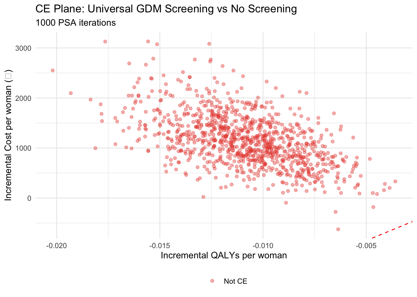
## 6. CE Plane and CEAC
```{r}
#| label: fig-ce-plane
#| echo: true
#| fig-cap: "Cost-effectiveness plane: Universal Screening vs No Screening (1,000 PSA iterations)"
library(ggplot2)
psa_results$ce <- psa_results$inc_nmb > 0

ggplot(psa_results, aes(x = inc_qaly, y = inc_cost, colour = ce)) +
  geom_point(alpha = 0.4, size = 1.5) +
  geom_abline(intercept = 0, slope = wtp_india, linetype = "dashed", colour = "red") +
  scale_colour_manual(values = c("TRUE" = "#2ecc71", "FALSE" = "#e74c3c"),
                      labels = c("TRUE" = "Cost-effective", "FALSE" = "Not CE"),
                      name = "") +
  labs(x = "Incremental QALYs per woman",
       y = "Incremental Cost per woman (₹)",
       title = "CE Plane: Universal GDM Screening vs No Screening",
       subtitle = paste(n_psa, "PSA iterations")) +
  theme_minimal() +
  theme(legend.position = "bottom")
```
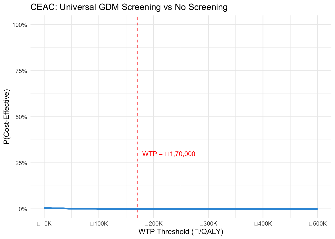
```{r}
#| label: fig-ceac
#| echo: true
#| fig-cap: "Cost-effectiveness acceptability curve"
wtp_range <- seq(0, 500000, by = 5000)
ceac <- sapply(wtp_range, function(w) {
  mean(w * psa_results$inc_qaly - psa_results$inc_cost > 0)
})

ceac_df <- data.frame(WTP = wtp_range, Prob_CE = ceac)

ggplot(ceac_df, aes(x = WTP, y = Prob_CE)) +
  geom_line(linewidth = 1.2, colour = "#3498db") +
  geom_ribbon(aes(ymin = 0, ymax = Prob_CE), alpha = 0.15, fill = "#3498db") +
  geom_vline(xintercept = wtp_india, linetype = "dashed", colour = "red") +
  annotate("text", x = wtp_india, y = 0.3, label = "WTP = ₹1,70,000",
           colour = "red", hjust = -0.1, size = 3.5) +
  scale_x_continuous(labels = function(x) paste0("₹", format(x/1000, big.mark = ","), "K")) +
  scale_y_continuous(limits = c(0, 1), labels = scales::percent) +
  labs(x = "WTP Threshold (₹/QALY)", y = "P(Cost-Effective)",
       title = "CEAC: Universal GDM Screening vs No Screening") +
  theme_minimal()
```
## 7. PSA Summary
```{r}
#| label: psa-summary
#| echo: true
kable(data.frame(
  Metric = c("Mean Incremental Cost/woman",
             "Mean Incremental QALYs/woman",
             "Mean Incremental NMB",
             paste0("P(cost-effective) at ₹", format(wtp_india, big.mark = ",")),
             "P(dominant)"),
  Value = c(
    paste0("₹", format(round(mean(psa_results$inc_cost)), big.mark = ",")),
    round(mean(psa_results$inc_qaly), 4),
    paste0("₹", format(round(mean(psa_results$inc_nmb)), big.mark = ",")),
    paste0(round(mean(psa_results$inc_nmb > 0) * 100, 1), "%"),
    paste0(round(mean(psa_results$inc_cost < 0 & psa_results$inc_qaly > 0) * 100, 1), "%")
  ),
  check.names = FALSE
), caption = paste0("PSA summary (", n_psa, " iterations)"))
```
## 8. What You Learned
This bonus page shows the same pattern you saw in Session 4 Bonus (rdecision for DES vs BMS) and Session 5 Bonus (heemod for Markov):
1. **Manual first, package second** — you built the diagnostic tree from scratch in Session 3, now you see it through a package lens
2. **Cross-validation** — the rdecision results should match the manual R model exactly
3. **PSA comes free** — once the tree is in rdecision, Monte Carlo simulation is straightforward
4. **NMB over ICER** — the PSA summary uses NMB, not averaged ICERs
The pattern is the same for all three model types: understand the mechanics manually, then use a validated package for production work.
## Key References
- Filipović-Pierucci A et al. Markov Models for Health Economic Evaluations: The R Package heemod. *arXiv*.
- Briggs A et al. (2006). Decision Modelling for Health Economic Evaluation. Oxford University Press.
- rdecision CRAN documentation: [https://cran.r-project.org/package=rdecision](https://cran.r-project.org/package=rdecision)
→ **Back to:** [Session 3: GDM Diagnostic Tree (Manual)](gdm-diagnostic-tree.qmd) | [Exercise](gdm-exercise.qmd)