---
title: "Session 8: Partitioned Survival Model — Trastuzumab for HER2+ Breast Cancer"
subtitle: "Survival curve fitting, extrapolation, and area-under-the-curve partitioning"
format:
html:
toc: true
code-fold: show
code-tools: true
---
## The Clinical Question
Breast cancer is the most common cancer among Indian women, accounting for 27% of all cancers. Among HER2-positive patients, adding trastuzumab to chemotherapy improves disease-free survival (DFS) by approximately 50% and overall survival (OS) by 30%.
However, trastuzumab is expensive — ₹50,000 to ₹1,00,000 per dose — and has been used in only about 8.6% of eligible Indian patients. A cost-effectiveness study from Tata Memorial Centre (Shrestha et al. 2020, JCO Global Oncology) found the ICER ranged from ₹1,34,413 to ₹1,78,877 per QALY depending on trial estimates used.
**The HTA question:** Is adjuvant trastuzumab (1 year) cost-effective compared to chemotherapy alone for HER2+ breast cancer in India, using a partitioned survival modelling approach?
## What Is a Partitioned Survival Model?
Unlike a Markov model (where you define transition probabilities between states), a **partitioned survival model** (PSM) directly uses survival curves to determine the proportion of patients in each health state at any given time.
For oncology, the three states are typically:
1. **Progression-Free (PF):** Alive without disease progression
2. **Progressed Disease (PD):** Alive but disease has progressed
3. **Dead**
At any time point *t*:
- **Proportion PF** = PFS(t) — the progression-free survival curve
- **Proportion Dead** = 1 - OS(t) — one minus the overall survival curve
- **Proportion PD** = OS(t) - PFS(t) — the difference between OS and PFS
This is the **area-under-the-curve** approach. The key advantage: you work directly with survival data from clinical trials rather than estimating transition probabilities.
```{r}
#| label: fig-psm-structure
#| echo: true
#| fig-cap: "Partitioned survival model: three health states derived from OS and PFS curves"
library(DiagrammeR)

grViz("
digraph psm_structure {
  graph [rankdir=LR, bgcolor='transparent', fontname='Helvetica', nodesep=0.6]
  node [fontname='Helvetica', fontsize=11, style='filled,rounded', shape=box]

  PF [label='Progression-Free\n(PF)\n\nProportion = PFS(t)\nUtility = 0.80\nCost varies by arm', fillcolor='#59a14f', fontcolor='white', width=2.5]
  PD [label='Progressed\nDisease (PD)\n\nProportion = OS(t) - PFS(t)\nUtility = 0.55\nCost = ₹1,80,000/yr', fillcolor='#f28e2b', fontcolor='white', width=2.5]
  Dead [label='Dead\n\nProportion = 1 - OS(t)\nUtility = 0\nCost = 0', fillcolor='#bab0ac', fontcolor='white', width=2.5, shape=doublecircle]

  PF -> PD [label='Progression']
  PD -> Dead [label='Death']
  PF -> Dead [label='Death\n(without progression)', style=dashed]
}
")
```
## Model Parameters
```{r}
#| label: parameters
#| echo: true
# ============================================================
# MODEL PARAMETERS — Breast Cancer Partitioned Survival Model
# ============================================================

# --- Time Horizon ---
time_horizon <- 20  # years (lifetime horizon for early breast cancer)
cycle_length <- 1   # annual cycles
n_cycles <- time_horizon / cycle_length
time_points <- seq(0, time_horizon, by = cycle_length)

# --- Survival Parameters ---
# We use Weibull distributions fitted to trial data
# PFS and OS for both arms
# Source: HERA trial (Camerini et al.); adapted with Indian survival
#         data from CONCORD study (5-year survival 66.1% in control)

# Weibull parameterisation: S(t) = exp(-lambda * t^gamma)
# lambda = scale parameter, gamma = shape parameter

# CHEMOTHERAPY ALONE (Control arm)
# OS: calibrated to 5-year survival ~66%, 10-year ~55%
os_lambda_control  <- 0.045
os_gamma_control   <- 1.15

# PFS: calibrated to median PFS ~4.5 years
pfs_lambda_control <- 0.12
pfs_gamma_control  <- 1.05

# TRASTUZUMAB + CHEMOTHERAPY (Intervention arm)
# OS: HR ~0.70 (30% reduction in mortality)
# PFS: HR ~0.50 (50% improvement in DFS)
# Applied as multiplicative effect on lambda
hr_os  <- 0.70
hr_pfs <- 0.50

os_lambda_intervention  <- os_lambda_control * hr_os
os_gamma_intervention   <- os_gamma_control

pfs_lambda_intervention <- pfs_lambda_control * hr_pfs
pfs_gamma_intervention  <- pfs_gamma_control

# --- Costs (₹ per year) ---
# Source: Tata Memorial Centre data; PMJAY rates; Shrestha et al. 2020
cost_pf_chemo  <- 25000     # Follow-up, routine monitoring (chemo alone)
cost_pf_trast  <- 420000    # Trastuzumab (year 1 only: ~6-8 doses) + monitoring
cost_pf_trast_maintenance <- 25000  # Years 2+ (same as chemo, trastuzumab stopped)
cost_pd        <- 180000    # Progressed disease: palliative care, second-line chemo
cost_dead      <- 0

# --- Utility Weights ---
# Source: Tata Memorial CEA; adapted from Beauchemin et al. 2014
utility_pf <- 0.80    # Progression-free
utility_pd <- 0.55    # Progressed disease
utility_dead <- 0.00

# --- Discount Rate ---
discount_rate <- 0.03
```
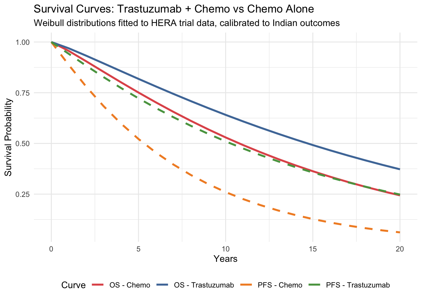
## Generating Survival Curves
```{r}
#| label: survival-curves
#| echo: true
#| fig-cap: "Overall survival and progression-free survival curves"
library(ggplot2)
# Weibull survival function: S(t) = exp(-lambda * t^gamma)
weibull_surv <- function(t, lambda, gamma) {
  exp(-lambda * t^gamma)
}

# Generate survival curves for both arms
surv_data <- data.frame(
  Time = rep(time_points, 4),
  Survival = c(
    weibull_surv(time_points, os_lambda_control, os_gamma_control),
    weibull_surv(time_points, os_lambda_intervention, os_gamma_intervention),
    weibull_surv(time_points, pfs_lambda_control, pfs_gamma_control),
    weibull_surv(time_points, pfs_lambda_intervention, pfs_gamma_intervention)
  ),
  Curve = rep(c("OS - Chemo", "OS - Trastuzumab",
                "PFS - Chemo", "PFS - Trastuzumab"), each = length(time_points)),
  Type = rep(c("OS", "OS", "PFS", "PFS"), each = length(time_points))
)

ggplot(surv_data, aes(x = Time, y = Survival, colour = Curve, linetype = Type)) +
  geom_line(linewidth = 1.1) +
  scale_colour_manual(values = c("OS - Chemo" = "#e15759",
                                  "OS - Trastuzumab" = "#4e79a7",
                                  "PFS - Chemo" = "#f28e2b",
                                  "PFS - Trastuzumab" = "#59a14f")) +
  scale_linetype_manual(values = c("OS" = "solid", "PFS" = "dashed")) +
  labs(
    x = "Years", y = "Survival Probability",
    title = "Survival Curves: Trastuzumab + Chemo vs Chemo Alone",
    subtitle = "Weibull distributions fitted to HERA trial data, calibrated to Indian outcomes"
  ) +
  theme_minimal() +
  theme(legend.position = "bottom") +
  guides(linetype = "none")
```
::: {.callout-tip}
## Reading These Curves
The higher a curve, the better the survival. Notice that trastuzumab shifts both curves upward — patients live longer (OS) and stay disease-free longer (PFS). The *area between* the OS and PFS curves for each strategy represents time spent in progressed disease.
:::
## Running the Partitioned Survival Model
```{r}
#| label: psm-calculation
#| echo: true
# --- Calculate state occupancy at each time point ---

# Control arm (Chemotherapy alone)
os_control  <- weibull_surv(time_points, os_lambda_control, os_gamma_control)
pfs_control <- weibull_surv(time_points, pfs_lambda_control, pfs_gamma_control)

# Ensure PFS never exceeds OS (logical constraint)
pfs_control <- pmin(pfs_control, os_control)

# State proportions at each time point
prop_pf_control   <- pfs_control
prop_pd_control   <- os_control - pfs_control
prop_dead_control <- 1 - os_control

# Intervention arm (Trastuzumab + Chemotherapy)
os_intervention  <- weibull_surv(time_points, os_lambda_intervention, os_gamma_intervention)
pfs_intervention <- weibull_surv(time_points, pfs_lambda_intervention, pfs_gamma_intervention)
pfs_intervention <- pmin(pfs_intervention, os_intervention)

prop_pf_intervention   <- pfs_intervention
prop_pd_intervention   <- os_intervention - pfs_intervention
prop_dead_intervention <- 1 - os_intervention

library(knitr)

# State occupancy at key time points
occ_table <- data.frame(
  Year = c(5, 10, 20, 5, 10, 20),
  Strategy = c(rep("Chemo Alone", 3), rep("Trastuzumab + Chemo", 3)),
  `Progression-Free` = c(
    round(prop_pf_control[6], 3), round(prop_pf_control[11], 3), round(prop_pf_control[21], 3),
    round(prop_pf_intervention[6], 3), round(prop_pf_intervention[11], 3), round(prop_pf_intervention[21], 3)
  ),
  `Progressed Disease` = c(
    round(prop_pd_control[6], 3), round(prop_pd_control[11], 3), round(prop_pd_control[21], 3),
    round(prop_pd_intervention[6], 3), round(prop_pd_intervention[11], 3), round(prop_pd_intervention[21], 3)
  ),
  Dead = c(
    round(prop_dead_control[6], 3), round(prop_dead_control[11], 3), round(prop_dead_control[21], 3),
    round(prop_dead_intervention[6], 3), round(prop_dead_intervention[11], 3), round(prop_dead_intervention[21], 3)
  ),
  check.names = FALSE
)

kable(occ_table, align = "clrrr",
      caption = "State occupancy (proportion) at key time points")
```
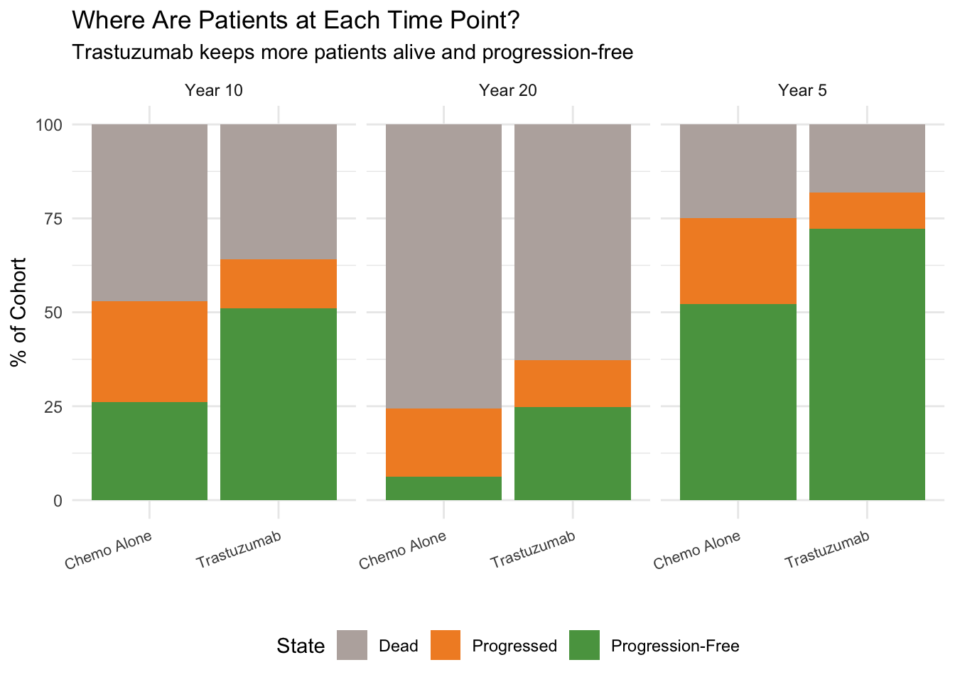
## State Occupancy at Key Timepoints
```{r}
#| label: fig-state-occupancy-bars
#| echo: true
#| fig-cap: "State occupancy at years 5, 10, and 20"
occ_data <- data.frame(
  Year = rep(c("Year 5", "Year 10", "Year 20"), each = 2),
  Strategy = rep(c("Chemo Alone", "Trastuzumab"), 3),
  PF = c(prop_pf_control[6], prop_pf_intervention[6],
         prop_pf_control[11], prop_pf_intervention[11],
         prop_pf_control[21], prop_pf_intervention[21]),
  PD = c(prop_pd_control[6], prop_pd_intervention[6],
         prop_pd_control[11], prop_pd_intervention[11],
         prop_pd_control[21], prop_pd_intervention[21]),
  Dead = c(prop_dead_control[6], prop_dead_intervention[6],
           prop_dead_control[11], prop_dead_intervention[11],
           prop_dead_control[21], prop_dead_intervention[21])
)

library(tidyr)
occ_long <- pivot_longer(occ_data, cols = c(PF, PD, Dead),
                          names_to = "State", values_to = "Proportion")
occ_long$State <- factor(occ_long$State, levels = c("Dead", "PD", "PF"))

ggplot(occ_long, aes(x = Strategy, y = Proportion * 100, fill = State)) +
  geom_col() +
  facet_wrap(~Year) +
  scale_fill_manual(values = c("PF" = "#59a14f", "PD" = "#f28e2b", "Dead" = "#bab0ac"),
                    labels = c("PF" = "Progression-Free", "PD" = "Progressed", "Dead" = "Dead")) +
  labs(x = "", y = "% of Cohort",
       title = "Where Are Patients at Each Time Point?",
       subtitle = "Trastuzumab keeps more patients alive and progression-free") +
  theme_minimal() +
  theme(legend.position = "bottom", axis.text.x = element_text(size = 8, angle = 20, hjust = 1))
```
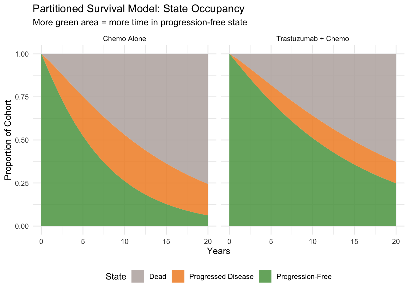
## Visualising State Occupancy
```{r}
#| label: state-occupancy-plot
#| echo: true
#| fig-cap: "State occupancy over time — partitioned survival approach"
library(tidyr)

# Prepare data for stacked area plot
state_data <- data.frame(
  Time = rep(time_points, 6),
  Proportion = c(
    prop_pf_control, prop_pd_control, prop_dead_control,
    prop_pf_intervention, prop_pd_intervention, prop_dead_intervention
  ),
  State = rep(rep(c("Progression-Free", "Progressed Disease", "Dead"),
                  each = length(time_points)), 2),
  Strategy = rep(c("Chemo Alone", "Trastuzumab + Chemo"),
                 each = 3 * length(time_points))
)

state_data$State <- factor(state_data$State,
                           levels = c("Dead", "Progressed Disease", "Progression-Free"))

ggplot(state_data, aes(x = Time, y = Proportion, fill = State)) +
  geom_area(alpha = 0.85) +
  facet_wrap(~Strategy) +
  scale_fill_manual(values = c("Progression-Free" = "#59a14f",
                                "Progressed Disease" = "#f28e2b",
                                "Dead" = "#bab0ac")) +
  labs(
    x = "Years", y = "Proportion of Cohort",
    title = "Partitioned Survival Model: State Occupancy",
    subtitle = "More green area = more time in progression-free state"
  ) +
  theme_minimal() +
  theme(legend.position = "bottom")
```
## Calculating Costs and QALYs
You already know these steps from the Markov model in Session 5: half-cycle correction, discounting, and cost/QALY accumulation. The only difference is that the "trace" comes from survival curves rather than matrix multiplication.
```{r}
#| label: costs-qalys
#| echo: true
# --- Half-cycle corrected state occupancy ---
# Same idea as Session 5: average proportion between start and end of each cycle
hcc_pf_control   <- (prop_pf_control[1:n_cycles] + prop_pf_control[2:(n_cycles+1)]) / 2
hcc_pd_control   <- (prop_pd_control[1:n_cycles] + prop_pd_control[2:(n_cycles+1)]) / 2

hcc_pf_intervention <- (prop_pf_intervention[1:n_cycles] + prop_pf_intervention[2:(n_cycles+1)]) / 2
hcc_pd_intervention <- (prop_pd_intervention[1:n_cycles] + prop_pd_intervention[2:(n_cycles+1)]) / 2

# --- Discount factors ---
discount_factors <- 1 / (1 + discount_rate)^(0:(n_cycles - 1))

# --- CONTROL ARM: Costs ---
# Same cost structure throughout
cost_per_cycle_control <- hcc_pf_control * cost_pf_chemo +
                          hcc_pd_control * cost_pd

total_cost_control <- sum(cost_per_cycle_control * discount_factors)

# --- INTERVENTION ARM: Costs ---
# Year 1: trastuzumab cost; Years 2+: maintenance only
cost_pf_by_year <- c(cost_pf_trast, rep(cost_pf_trast_maintenance, n_cycles - 1))

cost_per_cycle_intervention <- hcc_pf_intervention * cost_pf_by_year +
                               hcc_pd_intervention * cost_pd

total_cost_intervention <- sum(cost_per_cycle_intervention * discount_factors)

# --- QALYs ---
qaly_per_cycle_control <- hcc_pf_control * utility_pf + hcc_pd_control * utility_pd
qaly_per_cycle_intervention <- hcc_pf_intervention * utility_pf +
                               hcc_pd_intervention * utility_pd

total_qaly_control <- sum(qaly_per_cycle_control * discount_factors)
total_qaly_intervention <- sum(qaly_per_cycle_intervention * discount_factors)

kable(data.frame(
  Strategy = c("Chemo Alone", "Trastuzumab + Chemo"),
  `Discounted Cost (₹)` = c(
    paste0("₹", format(round(total_cost_control), big.mark = ",")),
    paste0("₹", format(round(total_cost_intervention), big.mark = ","))
  ),
  `Discounted QALYs` = c(
    round(total_qaly_control, 3),
    round(total_qaly_intervention, 3)
  ),
  check.names = FALSE
), align = "lrr",
   caption = "Discounted costs and QALYs per patient")
```
## ICER Calculation
```{r}
#| label: icer
#| echo: true
library(knitr)

inc_cost <- total_cost_intervention - total_cost_control
inc_qaly <- total_qaly_intervention - total_qaly_control
icer <- inc_cost / inc_qaly

# WTP threshold
wtp_india <- 170000
```
### Results Summary
```{r}
#| label: results-table
#| echo: true
kable(data.frame(
  Strategy = c("Chemo Alone", "Trastuzumab + Chemo", "Incremental"),
  `Total Cost (₹)` = c(
    paste0("₹", format(round(total_cost_control), big.mark = ",")),
    paste0("₹", format(round(total_cost_intervention), big.mark = ",")),
    paste0("₹", format(round(inc_cost), big.mark = ","))
  ),
  `Total QALYs` = c(
    round(total_qaly_control, 3),
    round(total_qaly_intervention, 3),
    round(inc_qaly, 3)
  ),
  check.names = FALSE
), align = "lrr",
   caption = "Cost-effectiveness results (20-year horizon, 3% discounting, per patient)")
```
### ICER Interpretation
```{r}
#| label: icer-interpretation
#| echo: true
# -------------------------------------------------------
# Handle the ICER carefully — check signs, not just the ratio
# -------------------------------------------------------
# Recall from Session 5: a negative ICER can mean DOMINANT or DOMINATED.
# Always check ΔCost and ΔQALYs separately.

interpretation <- if (inc_cost < 0 & inc_qaly > 0) {
  "DOMINANT — saves costs AND improves health"
} else if (inc_cost > 0 & inc_qaly < 0) {
  "DOMINATED — costs more AND worsens health"
} else if (inc_cost > 0 & inc_qaly > 0) {
  if (icer < wtp_india) {
    paste0("Cost-effective (ICER < WTP of ₹", format(wtp_india, big.mark = ","), ")")
  } else if (icer < 3 * wtp_india) {
    paste0("Cost-effective at 3× GDP/capita (₹", format(3 * wtp_india, big.mark = ","), ")")
  } else {
    "NOT cost-effective at conventional thresholds"
  }
} else {
  "Trade-off: saves money but loses QALYs"
}

kable(data.frame(
  Metric = c("Incremental Cost", "Incremental QALYs", "ICER",
             "WTP Threshold (1× GDP/capita)",
             "Published Indian ICER (Shrestha et al. 2020)", "Conclusion"),
  Value = c(
    paste0("₹", format(round(inc_cost), big.mark = ",")),
    round(inc_qaly, 3),
    paste0("₹", format(round(icer), big.mark = ","), " per QALY gained"),
    paste0("₹", format(wtp_india, big.mark = ",")),
    "₹1,34,413 to ₹1,78,877 per QALY",
    interpretation
  ),
  check.names = FALSE
), caption = "Cost-effectiveness conclusion")
```
### Net Monetary Benefit (NMB)
As we learned in Session 5, the ICER can be ambiguous when it's negative. The **Net Monetary Benefit** gives an unambiguous answer: positive ΔNMB = adopt.
```{r}
#| label: nmb
#| echo: true
# NMB = WTP × QALYs − Cost
nmb_control      <- wtp_india * total_qaly_control - total_cost_control
nmb_intervention <- wtp_india * total_qaly_intervention - total_cost_intervention
inc_nmb          <- nmb_intervention - nmb_control

kable(data.frame(
  Metric = c("NMB Chemo Alone", "NMB Trastuzumab + Chemo",
             "Incremental NMB (ΔNMB)", "Decision"),
  Value = c(
    paste0("₹", format(round(nmb_control), big.mark = ",")),
    paste0("₹", format(round(nmb_intervention), big.mark = ",")),
    paste0("₹", format(round(inc_nmb), big.mark = ",")),
    if (inc_nmb > 0) "ADOPT — positive ΔNMB" else "REJECT — negative ΔNMB"
  ),
  check.names = FALSE
), caption = paste0("Net Monetary Benefit (WTP = ₹", format(wtp_india, big.mark = ","), "/QALY)"))
```
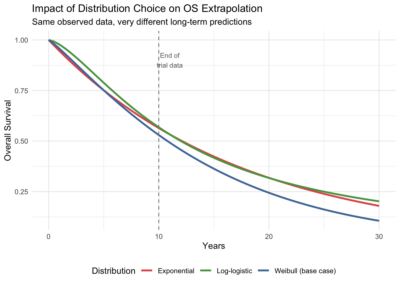
## The Crucial Role of Extrapolation
A critical feature of partitioned survival models is that survival curves must be **extrapolated** beyond the observed trial period. The choice of distribution dramatically affects the results.
```{r}
#| label: extrapolation-comparison
#| echo: true
#| fig-cap: "How distribution choice affects OS extrapolation"
# Compare Weibull, Exponential, and Log-logistic for control OS
t_extrap <- seq(0, 30, by = 0.5)

# Weibull (our base case)
os_weibull <- exp(-os_lambda_control * t_extrap^os_gamma_control)

# Exponential (constant hazard — simpler but often unrealistic)
# Calibrate to same 5-year survival
rate_exp <- -log(weibull_surv(5, os_lambda_control, os_gamma_control)) / 5
os_exponential <- exp(-rate_exp * t_extrap)

# Log-logistic (heavier tail — more optimistic long-term)
# Approximate calibration
ll_alpha <- 12
ll_beta  <- 1.5
os_loglogistic <- 1 / (1 + (t_extrap / ll_alpha)^ll_beta)

extrap_data <- data.frame(
  Time = rep(t_extrap, 3),
  Survival = c(os_weibull, os_exponential, os_loglogistic),
  Distribution = rep(c("Weibull (base case)", "Exponential", "Log-logistic"),
                     each = length(t_extrap))
)

ggplot(extrap_data, aes(x = Time, y = Survival, colour = Distribution)) +
  geom_line(linewidth = 1.1) +
  geom_vline(xintercept = 10, linetype = "dashed", colour = "grey50") +
  annotate("text", x = 11, y = 0.9, label = "End of\ntrial data",
           colour = "grey40", size = 3) +
  scale_colour_manual(values = c("Weibull (base case)" = "#4e79a7",
                                  "Exponential" = "#e15759",
                                  "Log-logistic" = "#59a14f")) +
  labs(
    x = "Years", y = "Overall Survival",
    title = "Impact of Distribution Choice on OS Extrapolation",
    subtitle = "Same observed data, very different long-term predictions"
  ) +
  theme_minimal() +
  theme(legend.position = "bottom")
```
::: {.callout-warning}
## Why Extrapolation Matters
Beyond the trial observation period (dashed line), the three distributions diverge dramatically. The log-logistic predicts much higher long-term survival than the Weibull or exponential. Since costs and QALYs accumulate over the entire time horizon, this choice alone can change the ICER by tens of thousands of rupees. **Always present results under multiple distributional assumptions** as a structural sensitivity analysis.
:::
## Life-Years and QALY Breakdown
```{r}
#| label: ly-breakdown
#| echo: true
# Total life-years (undiscounted) from the area under OS curve
ly_control <- sum((os_control[1:n_cycles] + os_control[2:(n_cycles+1)]) / 2)
ly_intervention <- sum((os_intervention[1:n_cycles] + os_intervention[2:(n_cycles+1)]) / 2)

# Time in PF (undiscounted)
pf_years_control <- sum(hcc_pf_control)
pf_years_intervention <- sum(hcc_pf_intervention)

# Time in PD (undiscounted)
pd_years_control <- sum(hcc_pd_control)
pd_years_intervention <- sum(hcc_pd_intervention)

kable(data.frame(
  Metric = c("Total life-years", "Years in PF", "Years in PD",
             "LY gained (intervention − control)", "PF years gained"),
  `Chemo Alone` = c(round(ly_control, 2), round(pf_years_control, 2),
                     round(pd_years_control, 2), "—", "—"),
  Trastuzumab = c(round(ly_intervention, 2), round(pf_years_intervention, 2),
                   round(pd_years_intervention, 2),
                   round(ly_intervention - ly_control, 2),
                   round(pf_years_intervention - pf_years_control, 2)),
  check.names = FALSE
), align = "lrr",
   caption = "Life-year and QALY breakdown (undiscounted, per patient)")
```
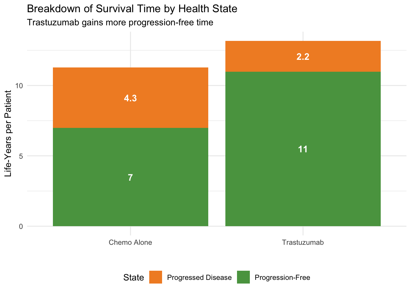
## Life-Years by Health State
```{r}
#| label: fig-ly-waterfall
#| echo: true
#| fig-cap: "Life-years in each state: Trastuzumab vs Chemo Alone"
ly_data <- data.frame(
  State = rep(c("Progression-Free", "Progressed Disease"), 2),
  Strategy = rep(c("Chemo Alone", "Trastuzumab"), each = 2),
  Years = c(pf_years_control, pd_years_control,
            pf_years_intervention, pd_years_intervention)
)

ggplot(ly_data, aes(x = Strategy, y = Years, fill = State)) +
  geom_col() +
  geom_text(aes(label = round(Years, 1)), position = position_stack(vjust = 0.5), size = 4, colour = "white", fontface = "bold") +
  scale_fill_manual(values = c("Progression-Free" = "#59a14f", "Progressed Disease" = "#f28e2b")) +
  labs(x = "", y = "Life-Years per Patient",
       title = "Breakdown of Survival Time by Health State",
       subtitle = "Trastuzumab gains more progression-free time") +
  theme_minimal() +
  theme(legend.position = "bottom")
```
## What You Just Did
You built a **partitioned survival model** — the standard approach for oncology HTA worldwide. Building on the Markov foundations from Session 5, the key *new* concepts were:
1. **Survival curve fitting** — using Weibull distributions to represent PFS and OS (replaces the transition matrix)
2. **State partitioning** — deriving health state occupancy directly from the relationship PD(t) = OS(t) − PFS(t)
3. **Area-under-the-curve** — the PSM equivalent of the Markov trace
4. **Extrapolation** — extending curves beyond trial data, where distribution choice alone can swing the ICER by tens of thousands of rupees
And the concepts that carried over unchanged from Session 5: half-cycle correction, discounting, ICER with proper 4-quadrant interpretation, and NMB for unambiguous decision-making.
The PSM is conceptually simpler than a Markov model for oncology because you work directly with trial survival data. However, it has limitations — it cannot easily model treatment switching, it assumes independence of PFS and OS transitions, and the extrapolation choice is often the single most influential assumption.
::: {.callout-note}
## PSM vs Markov: When to Use Which
Use **PSM** when you have good survival curve data from trials and the disease has a natural PF → PD → Dead trajectory (most solid tumors). Use **Markov** when you need to model complex transitions (e.g., relapse → remission → relapse), treatment switching, or when time-in-state matters for transition probabilities. Many real-world HTA submissions use both and cross-validate.
:::
## Key References
- Shrestha A et al. (2020). Cost effectiveness of trastuzumab for management of breast cancer in India. *JCO Global Oncology*.
- Cameron D et al. (2017). 11 years' follow-up of trastuzumab after adjuvant chemotherapy in HER2-positive early breast cancer (HERA trial). *Lancet*.
- CONCORD study. Global surveillance of trends in cancer survival.
- Tata Memorial Centre (2024). Evidence-based management of breast cancer. *Indian Journal of Cancer*.
- Beauchemin C et al. (2014). Cost-effectiveness of trastuzumab. Systematic review.
- NICE DSU Technical Support Documents on survival analysis for HTA.
→ **Next:** Open `breast-cancer-exercise.qmd` to explore how changing survival parameters and costs affects the results.