library(DiagrammeR)

grViz("
digraph psa_workflow {
  graph [rankdir=LR, bgcolor='transparent', fontname='Helvetica']
  node [shape=box, style='filled,rounded', fontname='Helvetica', fontsize=11]

  A [label='1. Define\nDistributions\nfor each parameter', fillcolor='#4e79a7', fontcolor='white']
  B [label='2. Sample\nParameters\n(random draw)', fillcolor='#59a14f', fontcolor='white']
  C [label='3. Run\nModel\n(one iteration)', fillcolor='#f28e2b', fontcolor='white']
  D [label='4. Store\nResults\n(cost, QALY, ICER)', fillcolor='#e15759', fontcolor='white']
  E [label='5. Repeat\n1000-10000\ntimes', fillcolor='#76b7b2', fontcolor='white']
  F [label='6. Summarise\nUncertainty\n(CE plane, CEAC)', fillcolor='#edc948', fontcolor='black']

  A -> B -> C -> D -> E -> F
  E -> B [style=dashed, label='Loop', fontsize=9]
}
")Session 6: Probabilistic Sensitivity Analysis
Why PSA matters and how R makes it practical
Why Probabilistic Sensitivity Analysis?
In health technology assessment, we rarely know parameter values with certainty. When you submitted a cost-effectiveness model to a journal or HTA agency using only point estimates—a single transition probability, a single cost, a single utility value—you were essentially claiming that these are the true values. But they are not. Every parameter carries uncertainty from the sources we used: clinical trials with limited sample sizes, cost data from particular regions, utility estimates that varied across populations.
Point estimates tell us what would happen if all parameters took their best-guess values simultaneously. But what if the true transition probability is slightly higher? What if costs are trending upward? What if the target population has lower health-related quality of life than the trial sample? Journals and HTA agencies—NICE, CADTH, India’s NITI Aayog, and others—now require that you demonstrate your results are robust to this uncertainty. They want to know: does your recommendation change if we vary the parameters within their plausible ranges? How confident can we really be?
This is where Probabilistic Sensitivity Analysis (PSA) steps in, and where R becomes genuinely powerful compared to Excel. In Excel, running 5,000 scenarios is tedious and error-prone: you either manage massive tables of random numbers or spend hours with Data Tables. In R, it is a few lines of code. You define your parameter distributions once, then sample thousands of times in a loop, recording the results. You get not just point estimates but probability distributions of your outcomes—and more importantly, you answer the real question: “Given all sources of parameter uncertainty, what is the probability that each strategy is cost-effective?”
Parameter Distributions in HTA
Different parameter types follow different distributions. Here is how to translate your uncertainties into statistical distributions that R can sample from.
grViz("
digraph dist_map {
  graph [rankdir=TB, bgcolor='transparent', fontname='Helvetica']
  node [fontname='Helvetica', fontsize=11, style='filled,rounded', shape=box]

  title [label='Parameter Type → Distribution', shape=none, fontsize=14, fontname='Helvetica-Bold']

  prob [label='Probabilities\n& Utilities\n(bounded 0-1)', fillcolor='#4e79a7', fontcolor='white', width=2]
  cost [label='Costs\n(non-negative,\nright-skewed)', fillcolor='#59a14f', fontcolor='white', width=2]
  hr [label='Hazard Ratios\n& Relative Risks\n(positive, often <1)', fillcolor='#f28e2b', fontcolor='white', width=2]

  beta [label='Beta(α, β)', fillcolor='#d4e6f1', shape=ellipse, width=1.5]
  gamma [label='Gamma(shape, rate)', fillcolor='#d5f5e3', shape=ellipse, width=1.5]
  lognorm [label='Log-Normal(μ, σ)', fillcolor='#fdebd0', shape=ellipse, width=1.5]

  title -> prob [style=invis]
  title -> cost [style=invis]
  title -> hr [style=invis]

  prob -> beta
  cost -> gamma
  hr -> lognorm
}
")Beta Distribution for Probabilities
Probabilities and proportions (transition probabilities, event rates) follow a Beta distribution. The Beta is bounded between 0 and 1, making it ideal.
Parameterisation from mean and SE:
If you have a transition probability with mean = 0.10 and standard error = 0.02, you can convert these to Beta parameters (α and β) using:
- α = μ × (μ(1-μ)/σ² - 1)
- β = (1-μ) × (μ(1-μ)/σ² - 1)
where μ is the mean and σ² is the variance (SE²).
R code example:
Gamma Distribution for Costs
Costs are non-negative and typically right-skewed (a few very expensive patients pull the mean upward). The Gamma distribution fits this well.
Parameterisation from mean and SE:
If costs have mean = ₹45,000 and SE = ₹5,000:
- shape = μ² / σ²
- rate = μ / σ²
R code example:
Log-Normal Distribution for Hazard Ratios
Hazard ratios, relative risks, and odds ratios are bounded at 0 and can be any positive value. The Log-Normal distribution is natural: the log of a log-normal is normal, and we typically report confidence intervals on the log scale.
Parameterisation from mean and 95% CI:
If a hazard ratio has point estimate = 0.66 with 95% CI (0.55, 0.79):
- The log(HR) follows Normal: log(0.66) ≈ -0.416
- The 95% CI on the log scale is [log(0.55), log(0.79)] ≈ [-0.598, -0.236]
- The SE on log scale ≈ (log upper - log lower) / 3.92
R code example:
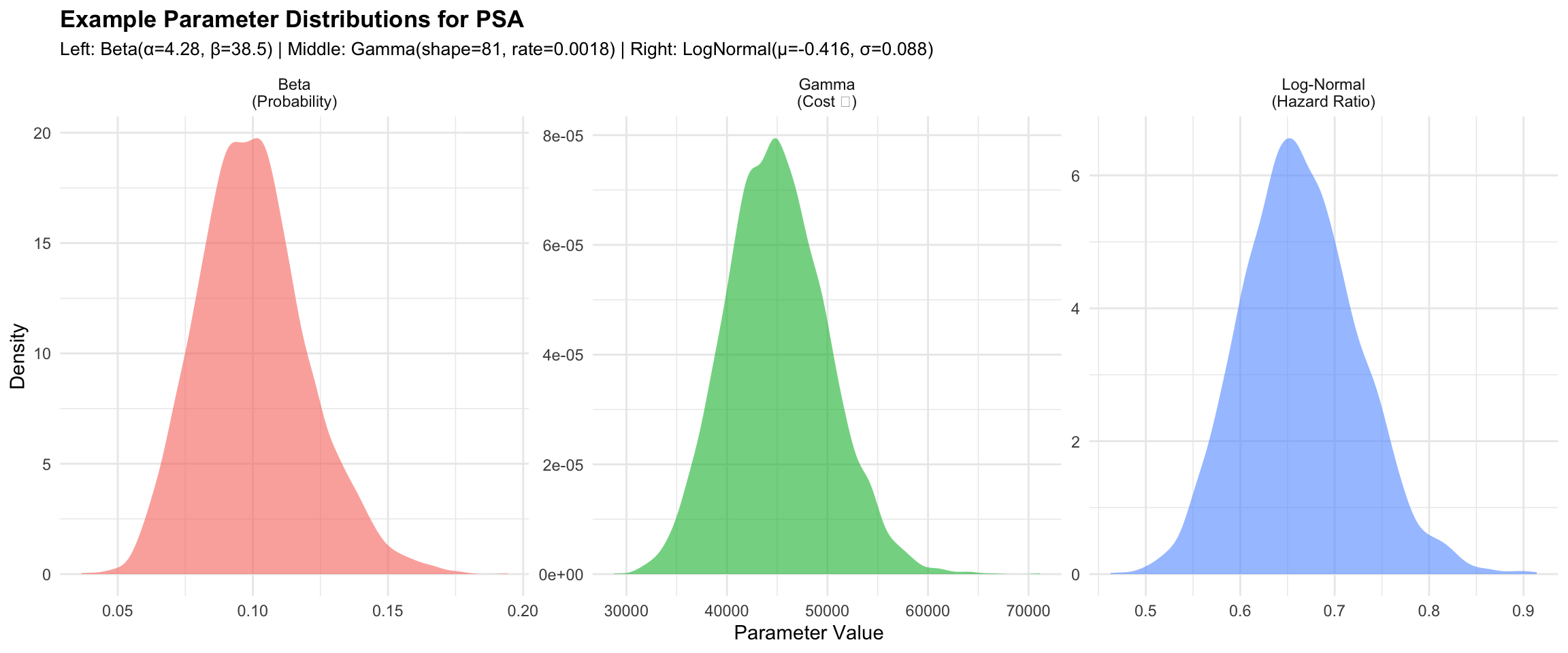
Visualising Example Distributions
Let us see what these distributions look like side-by-side:
Warning: package 'ggplot2' was built under R version 4.5.2library(dplyr)
library(tidyr)
# Set seed for reproducibility
set.seed(2026)
# Beta example: transition probability p_12 = 0.10, SE = 0.02
mean_p <- 0.10
se_p <- 0.02
var_p <- se_p^2
alpha_beta <- mean_p * (mean_p * (1 - mean_p) / var_p - 1)
beta_beta <- (1 - mean_p) * (mean_p * (1 - mean_p) / var_p - 1)
samples_beta <- rbeta(5000, alpha_beta, beta_beta)
# Gamma example: cost_moderate = ₹45,000, SE = ₹5,000
mean_cost <- 45000
se_cost <- 5000
shape_gamma <- mean_cost^2 / (se_cost^2)
rate_gamma <- mean_cost / (se_cost^2)
samples_gamma <- rgamma(5000, shape = shape_gamma, rate = rate_gamma)
# Log-Normal example: HR = 0.66, 95% CI (0.55, 0.79)
hr_point <- 0.66
hr_lower <- 0.55
hr_upper <- 0.79
log_hr_se <- (log(hr_upper) - log(hr_lower)) / 3.92
log_hr_mean <- log(hr_point)
samples_lognormal <- rlnorm(5000, meanlog = log_hr_mean, sdlog = log_hr_se)
# Combine into a single data frame for plotting
dist_data <- tibble(
Distribution = rep(c("Beta\n(Probability)", "Gamma\n(Cost ₹)", "Log-Normal\n(Hazard Ratio)"),
c(5000, 5000, 5000)),
Value = c(samples_beta, samples_gamma, samples_lognormal)
)
# Plot
ggplot(dist_data, aes(x = Value, fill = Distribution)) +
geom_density(alpha = 0.6, color = NA) +
facet_wrap(~ Distribution, scales = "free") +
labs(
title = "Example Parameter Distributions for PSA",
subtitle = "Left: Beta(α=4.28, β=38.5) | Middle: Gamma(shape=81, rate=0.0018) | Right: LogNormal(μ=-0.416, σ=0.088)",
x = "Parameter Value",
y = "Density"
) +
theme_minimal() +
theme(
legend.position = "none",
plot.title = element_text(face = "bold", size = 13),
plot.subtitle = element_text(size = 10)
)
PSA Applied to the CKD Markov Model
We’ll now run a full Probabilistic Sensitivity Analysis on the CKD model from Session 5. Recall the model structure:
- States: Early CKD (Stage 2) → Moderate CKD (Stage 3) → Advanced CKD / Dialysis (Stage 5) → Death
- Intervention: ACE inhibitor treatment (reduces progression by HR = 0.66)
- Cycle length: 1 year
- Time horizon: 20 years
Defining the PSA Function
Here is the core function that runs one iteration of the Markov model with a sampled parameter set:
run_markov_psa <- function(
    # Transition probabilities
    p_12, p_23, p_1d, p_2d, p_3d,
    # Treatment effect (hazard ratio for progression)
    hr_treatment,
    # Costs (annual, in Rupees)
    cost_early, cost_moderate, cost_advanced, cost_ace, cost_screening,
    # Utilities
    util_early, util_moderate, util_advanced,
    # Time horizon
    n_years = 20) {

  # Number of cohort members
  n_cohort <- 1000

  # Initialize states for standard care (no treatment)
  states_standard <- matrix(0, nrow = n_years + 1, ncol = 4)
  colnames(states_standard) <- c("Early", "Moderate", "Advanced", "Dead")

  # Initialize states for intervention (with treatment)
  states_intervention <- matrix(0, nrow = n_years + 1, ncol = 4)
  colnames(states_intervention) <- c("Early", "Moderate", "Advanced", "Dead")

  # Starting cohort: all in Early CKD state
  states_standard[1, 1] <- n_cohort
  states_intervention[1, 1] <- n_cohort

  # Run Markov chain for 20 years
  for (year in 1:n_years) {
    # Standard care: use base transition probabilities
    early_standard <- states_standard[year, 1]
    moderate_standard <- states_standard[year, 2]
    advanced_standard <- states_standard[year, 3]

    states_standard[year + 1, 1] <- early_standard * (1 - p_12 - p_1d)
    states_standard[year + 1, 2] <- early_standard * p_12 + moderate_standard * (1 - p_23 - p_2d)
    states_standard[year + 1, 3] <- moderate_standard * p_23 + advanced_standard * (1 - p_3d)
    states_standard[year + 1, 4] <- early_standard * p_1d +
                                     moderate_standard * p_2d +
                                     advanced_standard * p_3d +
                                     states_standard[year, 4]

    # Intervention: apply HR to progression probabilities
    early_intervention <- states_intervention[year, 1]
    moderate_intervention <- states_intervention[year, 2]
    advanced_intervention <- states_intervention[year, 3]

    # Reduced progression with HR
    p_12_tx <- 1 - (1 - p_12)^hr_treatment
    p_23_tx <- 1 - (1 - p_23)^hr_treatment

    states_intervention[year + 1, 1] <- early_intervention * (1 - p_12_tx - p_1d)
    states_intervention[year + 1, 2] <- early_intervention * p_12_tx +
                                         moderate_intervention * (1 - p_23_tx - p_2d)
    states_intervention[year + 1, 3] <- moderate_intervention * p_23_tx +
                                         advanced_intervention * (1 - p_3d)
    states_intervention[year + 1, 4] <- early_intervention * p_1d +
                                         moderate_intervention * p_2d +
                                         advanced_intervention * p_3d +
                                         states_intervention[year, 4]
  }

  # Calculate total costs and QALYs for standard care
  cost_standard <- sum(
    states_standard[-1, 1] * cost_early +
    states_standard[-1, 2] * cost_moderate +
    states_standard[-1, 3] * cost_advanced +
    states_standard[-1, 1] * cost_screening
  )

  qaly_standard <- sum(
    states_standard[-1, 1] * util_early +
    states_standard[-1, 2] * util_moderate +
    states_standard[-1, 3] * util_advanced
  )

  # Calculate total costs and QALYs for intervention
  cost_intervention <- sum(
    states_intervention[-1, 1] * cost_early +
    states_intervention[-1, 2] * cost_moderate +
    states_intervention[-1, 3] * cost_advanced +
    states_intervention[-1, 1] * cost_screening +
    states_intervention[-1, 1] * cost_ace
  )

  qaly_intervention <- sum(
    states_intervention[-1, 1] * util_early +
    states_intervention[-1, 2] * util_moderate +
    states_intervention[-1, 3] * util_advanced
  )

  return(list(
    cost_standard = cost_standard,
    cost_intervention = cost_intervention,
    qaly_standard = qaly_standard,
    qaly_intervention = qaly_intervention
  ))
}
Running the PSA: 5,000 Iterations
Now we define parameter distributions and run the PSA loop:
library(ggplot2)
library(dplyr)
library(tidyr)

set.seed(2026)

# Define parameter distributions
# ============================================================================

# Transition probabilities (Beta distributions)
# Base parameters from Session 5
p_12_mean <- 0.10
p_23_mean <- 0.12
p_1d_mean <- 0.02
p_2d_mean <- 0.04
p_3d_mean <- 0.15

# Standard errors (assumed from literature)
p_se <- 0.02  # Common SE for transition probabilities

# Convert to Beta parameters
convert_beta_params <- function(mean, se) {
  var <- se^2
  alpha <- mean * (mean * (1 - mean) / var - 1)
  beta <- (1 - mean) * (mean * (1 - mean) / var - 1)
  return(c(alpha = alpha, beta = beta))
}

beta_12 <- convert_beta_params(p_12_mean, p_se)
beta_23 <- convert_beta_params(p_23_mean, p_se)
beta_1d <- convert_beta_params(p_1d_mean, p_se)
beta_2d <- convert_beta_params(p_2d_mean, p_se)
beta_3d <- convert_beta_params(p_3d_mean, p_se)

# Treatment effect (Log-Normal): HR = 0.66, 95% CI (0.55, 0.79)
hr_mean <- 0.66
hr_lower <- 0.55
hr_upper <- 0.79
log_hr_se <- (log(hr_upper) - log(hr_lower)) / 3.92
log_hr_mean <- log(hr_mean)

# Costs (Gamma distributions)
# Base costs and standard errors
cost_early_mean <- 12000
cost_early_se <- 1500

cost_moderate_mean <- 45000
cost_moderate_se <- 5000

cost_advanced_mean <- 350000
cost_advanced_se <- 50000

cost_ace_mean <- 6000
cost_ace_se <- 800

cost_screening_mean <- 500
cost_screening_se <- 100

# Convert to Gamma parameters
convert_gamma_params <- function(mean, se) {
  var <- se^2
  shape <- mean^2 / var
  rate <- mean / var
  return(c(shape = shape, rate = rate))
}

gamma_early <- convert_gamma_params(cost_early_mean, cost_early_se)
gamma_moderate <- convert_gamma_params(cost_moderate_mean, cost_moderate_se)
gamma_advanced <- convert_gamma_params(cost_advanced_mean, cost_advanced_se)
gamma_ace <- convert_gamma_params(cost_ace_mean, cost_ace_se)
gamma_screening <- convert_gamma_params(cost_screening_mean, cost_screening_se)

# Utilities (Beta distributions)
# Utilities are proportions, so use Beta(α, β) directly
util_early_mean <- 0.85
util_early_se <- 0.05

util_moderate_mean <- 0.72
util_moderate_se <- 0.06

util_advanced_mean <- 0.55
util_advanced_se <- 0.08

beta_util_early <- convert_beta_params(util_early_mean, util_early_se)
beta_util_moderate <- convert_beta_params(util_moderate_mean, util_moderate_se)
beta_util_advanced <- convert_beta_params(util_advanced_mean, util_advanced_se)

# ============================================================================
# RUN PSA: 5,000 iterations
# ============================================================================

n_sim <- 5000
psa_results <- data.frame(
  iteration = 1:n_sim,
  cost_standard = NA,
  cost_intervention = NA,
  qaly_standard = NA,
  qaly_intervention = NA,
  inc_cost = NA,
  inc_qaly = NA,
  icer = NA
)

cat("Running CKD PSA...\n")
Running CKD PSA...for (i in 1:n_sim) {
# Sample parameters from distributions
p_12_sampled <- rbeta(1, beta_12["alpha"], beta_12["beta"])
p_23_sampled <- rbeta(1, beta_23["alpha"], beta_23["beta"])
p_1d_sampled <- rbeta(1, beta_1d["alpha"], beta_1d["beta"])
p_2d_sampled <- rbeta(1, beta_2d["alpha"], beta_2d["beta"])
p_3d_sampled <- rbeta(1, beta_3d["alpha"], beta_3d["beta"])
hr_sampled <- rlnorm(1, log_hr_mean, log_hr_se)
cost_early_sampled <- rgamma(1, gamma_early["shape"], gamma_early["rate"])
cost_moderate_sampled <- rgamma(1, gamma_moderate["shape"], gamma_moderate["rate"])
cost_advanced_sampled <- rgamma(1, gamma_advanced["shape"], gamma_advanced["rate"])
cost_ace_sampled <- rgamma(1, gamma_ace["shape"], gamma_ace["rate"])
cost_screening_sampled <- rgamma(1, gamma_screening["shape"], gamma_screening["rate"])
util_early_sampled <- rbeta(1, beta_util_early["alpha"], beta_util_early["beta"])
util_moderate_sampled <- rbeta(1, beta_util_moderate["alpha"], beta_util_moderate["beta"])
util_advanced_sampled <- rbeta(1, beta_util_advanced["alpha"], beta_util_advanced["beta"])
# Run model with sampled parameters
result <- run_markov_psa(
p_12 = p_12_sampled,
p_23 = p_23_sampled,
p_1d = p_1d_sampled,
p_2d = p_2d_sampled,
p_3d = p_3d_sampled,
hr_treatment = hr_sampled,
cost_early = cost_early_sampled,
cost_moderate = cost_moderate_sampled,
cost_advanced = cost_advanced_sampled,
cost_ace = cost_ace_sampled,
cost_screening = cost_screening_sampled,
util_early = util_early_sampled,
util_moderate = util_moderate_sampled,
util_advanced = util_advanced_sampled
)
# Store results
psa_results$cost_standard[i] <- result$cost_standard
psa_results$cost_intervention[i] <- result$cost_intervention
psa_results$qaly_standard[i] <- result$qaly_standard
psa_results$qaly_intervention[i] <- result$qaly_intervention
psa_results$inc_cost[i] <- result$cost_intervention - result$cost_standard
psa_results$inc_qaly[i] <- result$qaly_intervention - result$qaly_standard
psa_results$icer[i] <- psa_results$inc_cost[i] / psa_results$inc_qaly[i]
# Progress update
if (i %% 1000 == 0) {
cat(sprintf("Completed %d of %d iterations\n", i, n_sim))
}
}Completed 1000 of 5000 iterations
Completed 2000 of 5000 iterations
Completed 3000 of 5000 iterations
Completed 4000 of 5000 iterations
Completed 5000 of 5000 iterationsPSA complete.PSA Results Summary
library(knitr)

# Calculate summary statistics
mean_icer <- mean(psa_results$icer)
median_icer <- median(psa_results$icer)
lower_ci_icer <- quantile(psa_results$icer, 0.025)
upper_ci_icer <- quantile(psa_results$icer, 0.975)

mean_inc_cost <- mean(psa_results$inc_cost)
mean_inc_qaly <- mean(psa_results$inc_qaly)

# Create summary table
summary_table <- data.frame(
  Metric = c(
    "Mean Incremental Cost",
    "Mean Incremental QALY",
    "Mean ICER",
    "Median ICER",
    "95% Credible Interval (Lower)",
    "95% Credible Interval (Upper)",
    "WTP Threshold"
  ),
  Value = c(
    paste0("₹", format(round(mean_inc_cost), big.mark = ",")),
    format(round(mean_inc_qaly, 2), big.mark = ","),
    paste0("₹", format(round(mean_icer), big.mark = ","), "/QALY"),
    paste0("₹", format(round(median_icer), big.mark = ","), "/QALY"),
    paste0("₹", format(round(lower_ci_icer), big.mark = ",")),
    paste0("₹", format(round(upper_ci_icer), big.mark = ",")),
    "₹170,000/QALY"
  )
)

kable(summary_table,
      caption = "CKD Markov Model PSA Results (5,000 iterations)",
format = "html")| Metric | Value |
|---|---|
| Mean Incremental Cost | ₹-246,385,947 |
| Mean Incremental QALY | 1,152.77 |
| Mean ICER | ₹-240,731/QALY |
| Median ICER | ₹-209,298/QALY |
| 95% Credible Interval (Lower) | ₹-537,569 |
| 95% Credible Interval (Upper) | ₹-101,408 |
| WTP Threshold | ₹170,000/QALY |
# Filter out extreme ICERs for better visualisation
icer_filtered <- psa_results$icer[psa_results$icer > quantile(psa_results$icer, 0.01) &
                                   psa_results$icer < quantile(psa_results$icer, 0.99)]

ggplot(data.frame(ICER = icer_filtered), aes(x = ICER)) +
  geom_histogram(bins = 50, fill = "steelblue", colour = "white", alpha = 0.8) +
  geom_vline(xintercept = 170000, colour = "red", linetype = "dashed", linewidth = 1) +
  annotate("text", x = 170000, y = Inf, label = "WTP = ₹170,000/QALY",
           colour = "red", hjust = -0.1, vjust = 2, size = 3.5) +
  geom_vline(xintercept = mean(psa_results$icer), colour = "darkblue", linewidth = 1) +
  annotate("text", x = mean(psa_results$icer), y = Inf, label = "Mean ICER",
           colour = "darkblue", hjust = -0.1, vjust = 4, size = 3.5) +
  scale_x_continuous(labels = function(x) paste0("₹", format(round(x/1000), big.mark=","), "K")) +
  labs(x = "ICER (₹/QALY)", y = "Frequency",
       title = "Distribution of ICER Estimates",
       subtitle = "CKD Markov Model — 5,000 PSA iterations") +
  theme_minimal()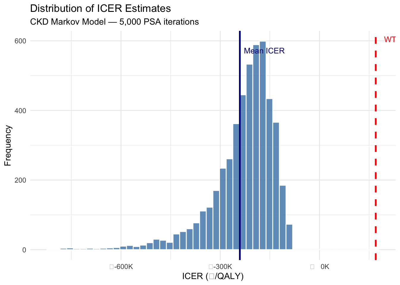
PSA Visualisations: Cost-Effectiveness Plane
The cost-effectiveness plane shows all 5,000 PSA iterations as points. The x-axis is incremental QALYs (our model gains QALYs with treatment), and the y-axis is incremental costs.
- Points in the bottom-right quadrant are dominant: more effective AND cheaper.
- Points in the top-right quadrant are cost-effective if they fall below the WTP line.
- Points in the top-left quadrant are dominated: more costly but less effective.
# Add WTP line parameter
wtp <- 170000  # ₹170,000 per QALY

# Create the cost-effectiveness plane
ce_plane <- ggplot(psa_results, aes(x = inc_qaly, y = inc_cost)) +
  # Add WTP line
  geom_abline(intercept = 0, slope = wtp, color = "red", linewidth = 1, linetype = "dashed",
              label = paste("WTP threshold: ₹", format(wtp, big.mark=","), "/QALY")) +
  # Add data points
  geom_point(alpha = 0.4, color = "steelblue", size = 2) +
  # Add quadrant lines
  geom_hline(yintercept = 0, color = "gray70", linewidth = 0.5) +
  geom_vline(xintercept = 0, color = "gray70", linewidth = 0.5) +
  # Labels and formatting
  labs(
    title = "Cost-Effectiveness Plane: CKD Markov Model PSA",
    subtitle = paste(n_sim, "iterations"),
    x = "Incremental QALYs (Intervention vs Standard Care)",
    y = "Incremental Cost (₹)",
    caption = "Red dashed line = ₹170,000/QALY willingness-to-pay threshold"
  ) +
  scale_y_continuous(labels = scales::comma_format(prefix = "₹")) +
  scale_x_continuous(labels = scales::comma_format()) +
  theme_minimal() +
  theme(
    plot.title = element_text(face = "bold", size = 13),
    plot.subtitle = element_text(size = 11),
    panel.grid.major = element_line(color = "gray95"),
    legend.position = "top"
  )
Warning in geom_abline(intercept = 0, slope = wtp, color = "red", linewidth =
1, : Ignoring unknown parameters: `label`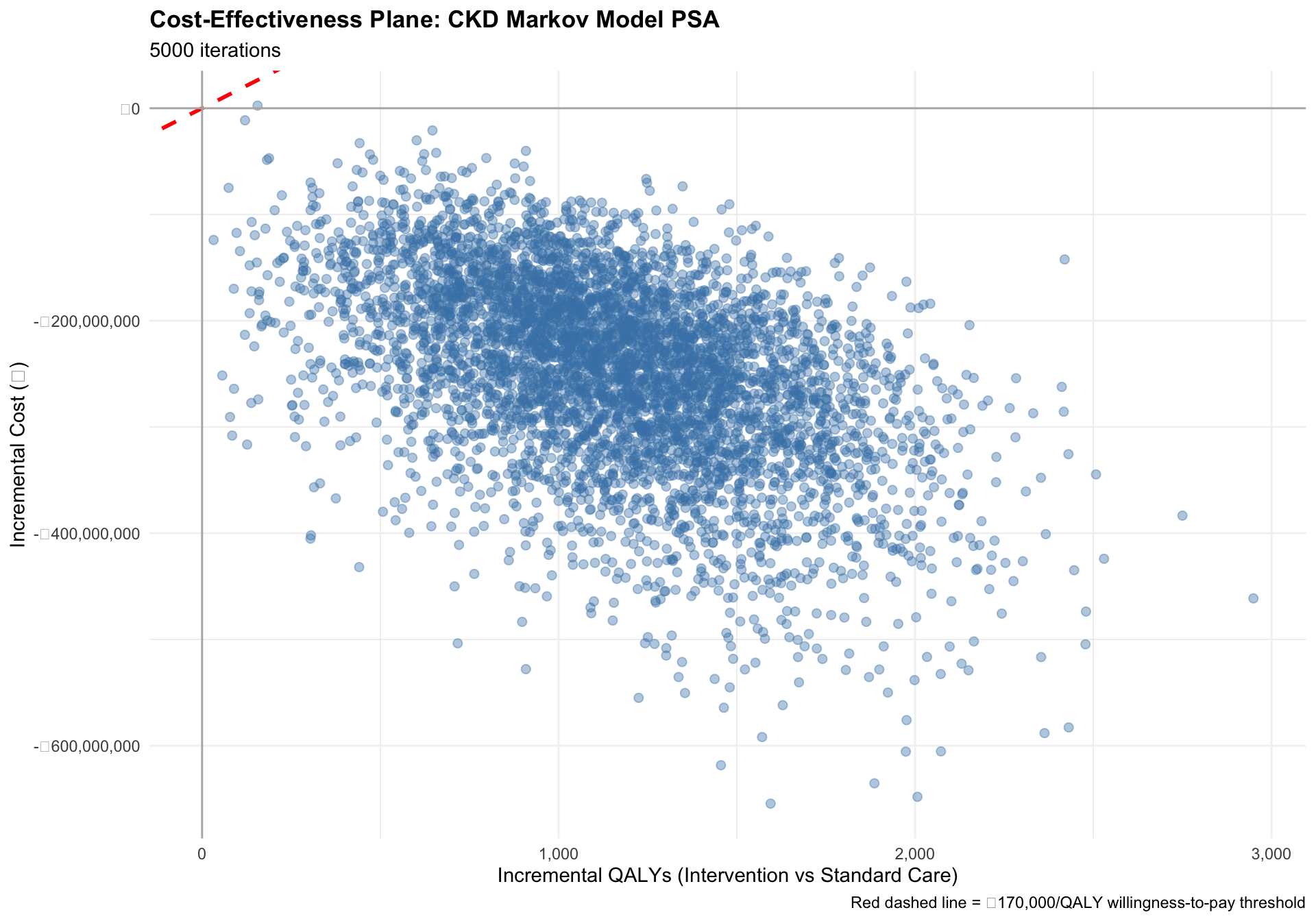
Cost-Effectiveness Acceptability Curve (CEAC)
The CEAC answers the question: “Across a range of willingness-to-pay thresholds, what is the probability that the intervention is cost-effective?” It is calculated by determining, for each WTP threshold, what proportion of the 5,000 PSA iterations had an ICER below that threshold.
# Define a range of WTP thresholds
wtp_range <- seq(0, 500000, by = 10000)

# For each WTP, calculate probability that intervention is cost-effective
ceac_data <- data.frame(
  wtp = wtp_range,
  prob_cost_effective = NA
)

for (j in 1:nrow(ceac_data)) {
  # Net Monetary Benefit (NMB) for intervention at each WTP:
  # NMB = (inc_qaly * wtp) - inc_cost
  nmb_intervention <- psa_results$inc_qaly * ceac_data$wtp[j] - psa_results$inc_cost

  # Probability that NMB > 0 (i.e., intervention is cost-effective)
  ceac_data$prob_cost_effective[j] <- mean(nmb_intervention > 0)
}

# Plot CEAC
ceac_plot <- ggplot(ceac_data, aes(x = wtp, y = prob_cost_effective)) +
  geom_line(color = "steelblue", linewidth = 1) +
  geom_area(fill = "steelblue", alpha = 0.3) +
  # Add reference line at WTP = 170,000
  geom_vline(xintercept = 170000, color = "red", linetype = "dashed", linewidth = 1) +
  # Labels and formatting
  labs(
    title = "Cost-Effectiveness Acceptability Curve (CEAC): CKD Markov Model",
    subtitle = paste(n_sim, "PSA iterations"),
    x = "Willingness-to-Pay Threshold (₹ per QALY)",
    y = "Probability That Intervention is Cost-Effective",
    caption = "Red dashed line = ₹170,000/QALY threshold"
  ) +
  scale_x_continuous(labels = scales::comma_format(prefix = "₹")) +
  scale_y_continuous(limits = c(0, 1), labels = scales::percent_format()) +
  theme_minimal() +
  theme(
    plot.title = element_text(face = "bold", size = 13),
    plot.subtitle = element_text(size = 11),
    panel.grid.major = element_line(color = "gray95")
  )

print(ceac_plot)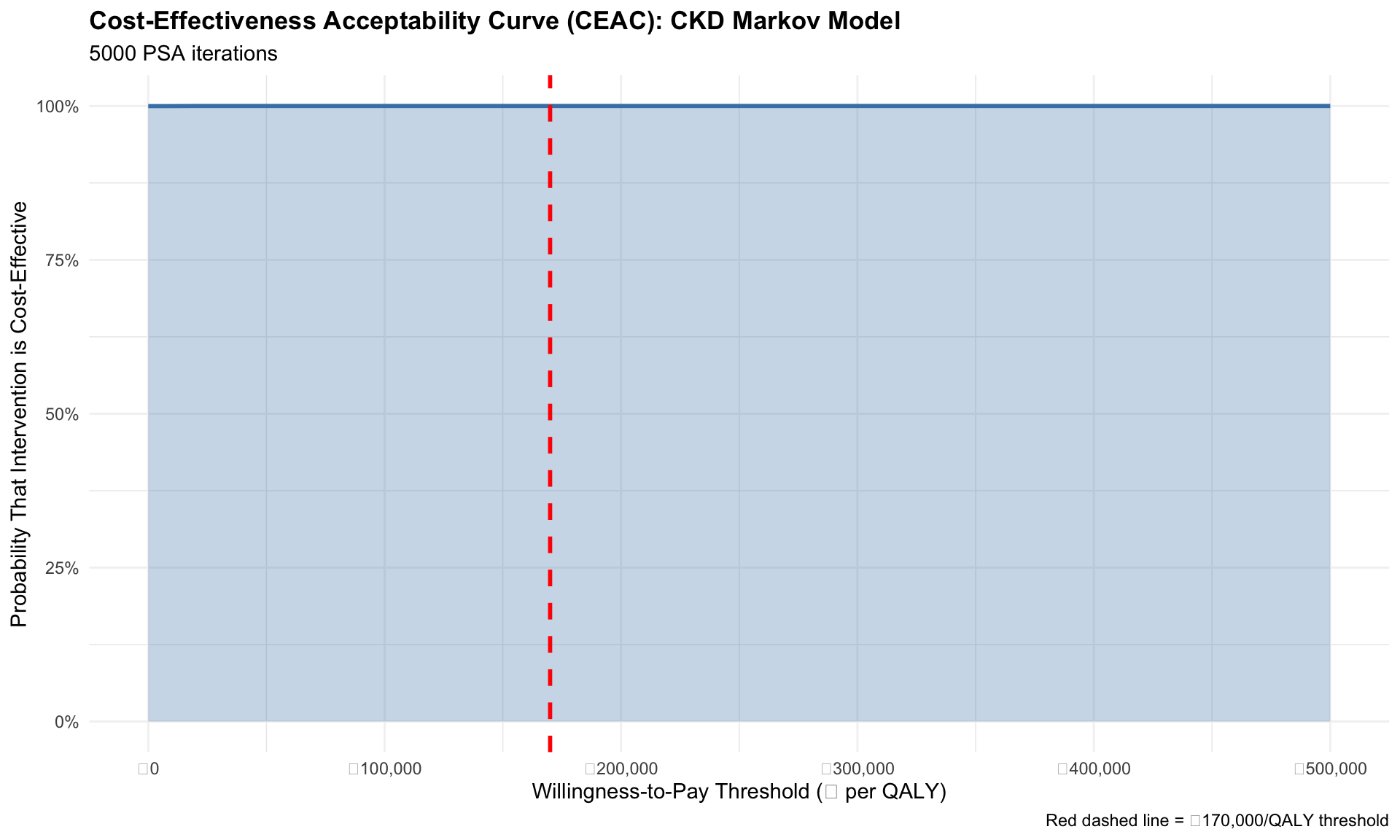
# Calculate probability at the ₹170,000 threshold
wtp_threshold <- 170000
nmb_at_threshold <- psa_results$inc_qaly * wtp_threshold - psa_results$inc_cost
prob_ce_at_170k <- mean(nmb_at_threshold > 0)
mean_nmb_at_170k <- mean(nmb_at_threshold)
lower_ci_nmb <- quantile(nmb_at_threshold, 0.025)
upper_ci_nmb <- quantile(nmb_at_threshold, 0.975)

# Create summary table for NMB at WTP threshold
nmb_summary <- data.frame(
  Metric = c(
    "Willingness-to-Pay Threshold",
    "Mean Net Monetary Benefit (NMB)",
    "Probability Cost-Effective",
    "95% CI for NMB (Lower)",
    "95% CI for NMB (Upper)"
  ),
  Value = c(
    paste0("₹", format(wtp_threshold, big.mark = ",")),
    paste0("₹", format(round(mean_nmb_at_170k), big.mark = ",")),
    paste0(sprintf("%.1f%%", prob_ce_at_170k * 100)),
    paste0("₹", format(round(lower_ci_nmb), big.mark = ",")),
    paste0("₹", format(round(upper_ci_nmb), big.mark = ","))
  )
)

kable(nmb_summary,
      caption = "Net Monetary Benefit Analysis at WTP = ₹170,000/QALY",
format = "html")| Metric | Value |
|---|---|
| Willingness-to-Pay Threshold | ₹170,000 |
| Mean Net Monetary Benefit (NMB) | ₹442,356,457 |
| Probability Cost-Effective | 100.0% |
| 95% CI for NMB (Lower) | ₹201,129,869 |
| 95% CI for NMB (Upper) | ₹732,063,347 |
PSA Applied to DES vs BMS Decision Tree
We can apply the same PSA logic to the DES vs BMS comparison from Session 4. The model is simpler (a decision tree with no transitions over time), but the principle is identical: define parameter distributions, sample 5,000 times, and visualise uncertainty.
Setup: DES vs BMS PSA Function
run_des_bms_psa <- function(
    # Clinical parameters
    p_mace_bms, p_mace_des,
    p_ist_bms, p_ist_des,
    # Costs (in Rupees)
    cost_bms, cost_des, cost_mace, cost_ist,
    # Utilities (quality-adjusted life expectancy, QALYs over model horizon)
    util_base, util_post_mace) {

  n_cohort <- 1000

  # BMS arm
  n_bms_mace <- n_cohort * p_mace_bms
  n_bms_ist <- n_cohort * p_ist_bms
  n_bms_uncomplicated <- n_cohort - n_bms_mace - n_bms_ist

  cost_bms_total <- n_cohort * cost_bms +
                    n_bms_mace * cost_mace +
                    n_bms_ist * cost_ist

  qaly_bms_total <- n_bms_uncomplicated * util_base +
                    n_bms_mace * util_post_mace +
                    n_bms_ist * util_post_mace

  # DES arm
  n_des_mace <- n_cohort * p_mace_des
  n_des_ist <- n_cohort * p_ist_des
  n_des_uncomplicated <- n_cohort - n_des_mace - n_des_ist

  cost_des_total <- n_cohort * cost_des +
                    n_des_mace * cost_mace +
                    n_des_ist * cost_ist

  qaly_des_total <- n_des_uncomplicated * util_base +
                    n_des_mace * util_post_mace +
                    n_des_ist * util_post_mace

  return(list(
    cost_bms = cost_bms_total,
    cost_des = cost_des_total,
    qaly_bms = qaly_bms_total,
    qaly_des = qaly_des_total
  ))
}
Running DES vs BMS PSA
set.seed(2026)

# Define parameter distributions for DES vs BMS
# ============================================================================

# Event rates (Beta distributions)
p_mace_bms_mean <- 0.12
p_mace_des_mean <- 0.08
p_ist_bms_mean <- 0.05
p_ist_des_mean <- 0.02

p_se <- 0.02

beta_mace_bms <- convert_beta_params(p_mace_bms_mean, p_se)
beta_mace_des <- convert_beta_params(p_mace_des_mean, p_se)
beta_ist_bms <- convert_beta_params(p_ist_bms_mean, p_se)
beta_ist_des <- convert_beta_params(p_ist_des_mean, p_se)

# Costs (Gamma distributions)
cost_bms_mean <- 200000
cost_bms_se <- 20000

cost_des_mean <- 320000
cost_des_se <- 30000

cost_mace_mean <- 150000
cost_mace_se <- 25000

cost_ist_mean <- 50000
cost_ist_se <- 10000

gamma_cost_bms <- convert_gamma_params(cost_bms_mean, cost_bms_se)
gamma_cost_des <- convert_gamma_params(cost_des_mean, cost_des_se)
gamma_cost_mace <- convert_gamma_params(cost_mace_mean, cost_mace_se)
gamma_cost_ist <- convert_gamma_params(cost_ist_mean, cost_ist_se)

# Utilities (Beta distributions)
util_base_mean <- 0.92
util_base_se <- 0.03

util_post_mace_mean <- 0.70
util_post_mace_se <- 0.05

beta_util_base <- convert_beta_params(util_base_mean, util_base_se)
beta_util_post_mace <- convert_beta_params(util_post_mace_mean, util_post_mace_se)

# ============================================================================
# RUN PSA: 5,000 iterations
# ============================================================================

n_sim_des_bms <- 5000
psa_des_bms <- data.frame(
  iteration = 1:n_sim_des_bms,
  cost_bms = NA,
  cost_des = NA,
  qaly_bms = NA,
  qaly_des = NA,
  inc_cost = NA,
  inc_qaly = NA,
  icer = NA
)

cat("Running DES vs BMS PSA...\n")
Running DES vs BMS PSA...for (i in 1:n_sim_des_bms) {
# Sample parameters
p_mace_bms_samp <- rbeta(1, beta_mace_bms["alpha"], beta_mace_bms["beta"])
p_mace_des_samp <- rbeta(1, beta_mace_des["alpha"], beta_mace_des["beta"])
p_ist_bms_samp <- rbeta(1, beta_ist_bms["alpha"], beta_ist_bms["beta"])
p_ist_des_samp <- rbeta(1, beta_ist_des["alpha"], beta_ist_des["beta"])
cost_bms_samp <- rgamma(1, gamma_cost_bms["shape"], gamma_cost_bms["rate"])
cost_des_samp <- rgamma(1, gamma_cost_des["shape"], gamma_cost_des["rate"])
cost_mace_samp <- rgamma(1, gamma_cost_mace["shape"], gamma_cost_mace["rate"])
cost_ist_samp <- rgamma(1, gamma_cost_ist["shape"], gamma_cost_ist["rate"])
util_base_samp <- rbeta(1, beta_util_base["alpha"], beta_util_base["beta"])
util_post_mace_samp <- rbeta(1, beta_util_post_mace["alpha"], beta_util_post_mace["beta"])
# Run model
result_des_bms <- run_des_bms_psa(
p_mace_bms = p_mace_bms_samp,
p_mace_des = p_mace_des_samp,
p_ist_bms = p_ist_bms_samp,
p_ist_des = p_ist_des_samp,
cost_bms = cost_bms_samp,
cost_des = cost_des_samp,
cost_mace = cost_mace_samp,
cost_ist = cost_ist_samp,
util_base = util_base_samp,
util_post_mace = util_post_mace_samp
)
psa_des_bms$cost_bms[i] <- result_des_bms$cost_bms
psa_des_bms$cost_des[i] <- result_des_bms$cost_des
psa_des_bms$qaly_bms[i] <- result_des_bms$qaly_bms
psa_des_bms$qaly_des[i] <- result_des_bms$qaly_des
psa_des_bms$inc_cost[i] <- result_des_bms$cost_des - result_des_bms$cost_bms
psa_des_bms$inc_qaly[i] <- result_des_bms$qaly_des - result_des_bms$qaly_bms
psa_des_bms$icer[i] <- psa_des_bms$inc_cost[i] / psa_des_bms$inc_qaly[i]
if (i %% 1000 == 0) {
cat(sprintf("Completed %d of %d iterations\n", i, n_sim_des_bms))
}
}Completed 1000 of 5000 iterations
Completed 2000 of 5000 iterations
Completed 3000 of 5000 iterations
Completed 4000 of 5000 iterations
Completed 5000 of 5000 iterationsDES vs BMS PSA complete.DES vs BMS Results: CE Plane and CEAC
# CE Plane for DES vs BMS
ce_plane_des_bms <- ggplot(psa_des_bms, aes(x = inc_qaly, y = inc_cost)) +
  geom_abline(intercept = 0, slope = 170000, color = "red", linewidth = 1, linetype = "dashed") +
  geom_point(alpha = 0.4, color = "darkgreen", size = 2) +
  geom_hline(yintercept = 0, color = "gray70", linewidth = 0.5) +
  geom_vline(xintercept = 0, color = "gray70", linewidth = 0.5) +
  labs(
    title = "Cost-Effectiveness Plane: DES vs BMS",
    subtitle = paste(n_sim_des_bms, "PSA iterations"),
    x = "Incremental QALYs (DES vs BMS)",
    y = "Incremental Cost (₹)"
  ) +
  scale_y_continuous(labels = scales::comma_format(prefix = "₹")) +
  scale_x_continuous(labels = scales::comma_format()) +
  theme_minimal() +
  theme(
    plot.title = element_text(face = "bold", size = 13),
    panel.grid.major = element_line(color = "gray95")
  )

# CEAC for DES vs BMS
wtp_range_des_bms <- seq(0, 500000, by = 10000)
ceac_data_des_bms <- data.frame(
  wtp = wtp_range_des_bms,
  prob_cost_effective = NA
)

for (j in 1:nrow(ceac_data_des_bms)) {
  nmb_des <- psa_des_bms$inc_qaly * ceac_data_des_bms$wtp[j] - psa_des_bms$inc_cost
  ceac_data_des_bms$prob_cost_effective[j] <- mean(nmb_des > 0)
}

ceac_plot_des_bms <- ggplot(ceac_data_des_bms, aes(x = wtp, y = prob_cost_effective)) +
  geom_line(color = "darkgreen", linewidth = 1) +
  geom_area(fill = "darkgreen", alpha = 0.3) +
  geom_vline(xintercept = 170000, color = "red", linetype = "dashed", linewidth = 1) +
  labs(
    title = "CEAC: DES vs BMS",
    subtitle = paste(n_sim_des_bms, "PSA iterations"),
    x = "Willingness-to-Pay Threshold (₹ per QALY)",
    y = "Probability That DES is Cost-Effective"
  ) +
  scale_x_continuous(labels = scales::comma_format(prefix = "₹")) +
  scale_y_continuous(limits = c(0, 1), labels = scales::percent_format()) +
  theme_minimal() +
  theme(
    plot.title = element_text(face = "bold", size = 13),
    panel.grid.major = element_line(color = "gray95")
  )

# Print side-by-side
library(gridExtra)
grid.arrange(ce_plane_des_bms, ceac_plot_des_bms, ncol = 2)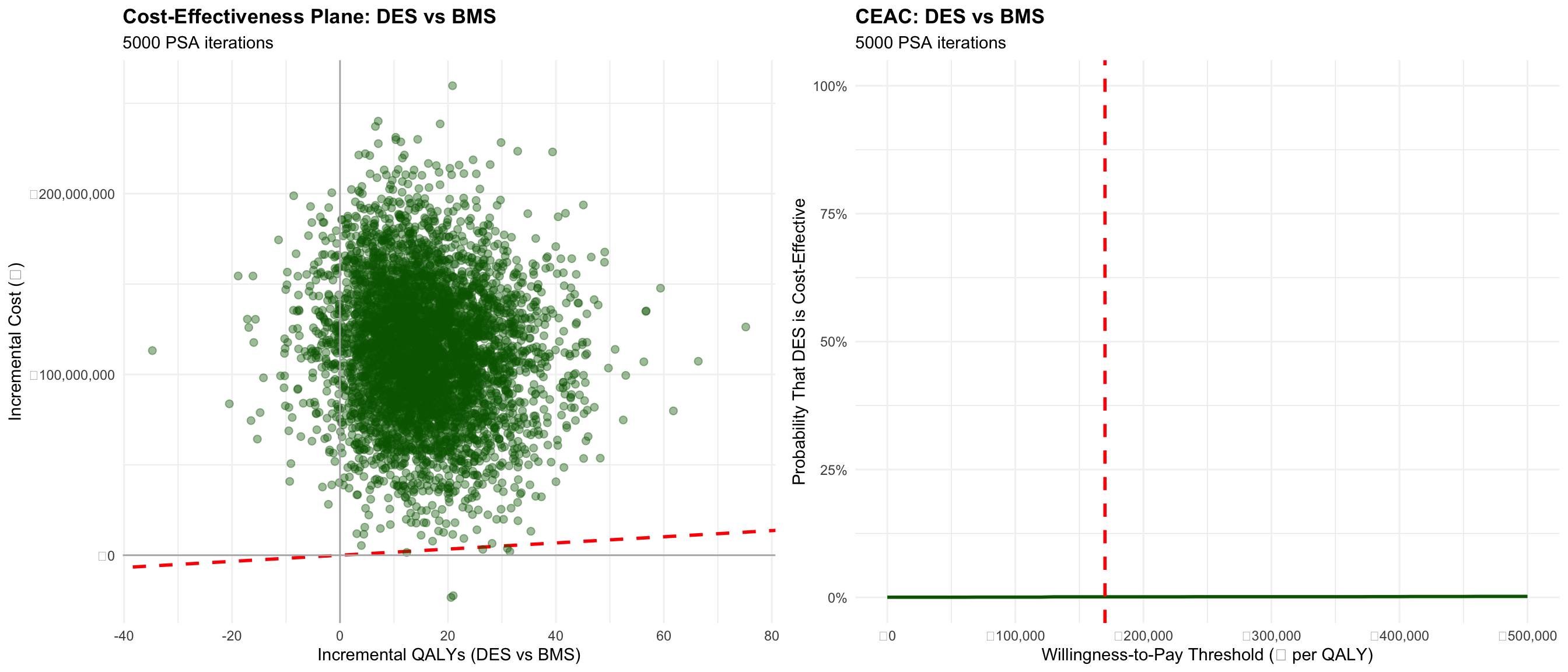
# Summary table
mean_icer_des_bms <- mean(psa_des_bms$icer)
median_icer_des_bms <- median(psa_des_bms$icer)
lower_ci_icer_des_bms <- quantile(psa_des_bms$icer, 0.025)
upper_ci_icer_des_bms <- quantile(psa_des_bms$icer, 0.975)

mean_inc_cost_des_bms <- mean(psa_des_bms$inc_cost)
mean_inc_qaly_des_bms <- mean(psa_des_bms$inc_qaly)

prob_des_ce_at_170k <- mean((psa_des_bms$inc_qaly * 170000 - psa_des_bms$inc_cost) > 0)
nmb_des_at_170k <- psa_des_bms$inc_qaly * 170000 - psa_des_bms$inc_cost
mean_nmb_des_170k <- mean(nmb_des_at_170k)

summary_table_des_bms <- data.frame(
  Metric = c(
    "Mean Incremental Cost",
    "Mean Incremental QALY",
    "Mean ICER",
    "Median ICER",
    "95% Credible Interval (Lower)",
    "95% Credible Interval (Upper)",
    "Mean NMB at ₹170,000/QALY",
    "Probability Cost-Effective at ₹170,000/QALY"
  ),
  Value = c(
    paste0("₹", format(round(mean_inc_cost_des_bms), big.mark = ",")),
    format(round(mean_inc_qaly_des_bms, 2), big.mark = ","),
    paste0("₹", format(round(mean_icer_des_bms), big.mark = ","), "/QALY"),
    paste0("₹", format(round(median_icer_des_bms), big.mark = ","), "/QALY"),
    paste0("₹", format(round(lower_ci_icer_des_bms), big.mark = ",")),
    paste0("₹", format(round(upper_ci_icer_des_bms), big.mark = ",")),
    paste0("₹", format(round(mean_nmb_des_170k), big.mark = ",")),
    paste0(sprintf("%.1f%%", prob_des_ce_at_170k * 100))
  )
)

kable(summary_table_des_bms,
      caption = "DES vs BMS PSA Results (5,000 iterations)",
format = "html")| Metric | Value |
|---|---|
| Mean Incremental Cost | ₹113,083,747 |
| Mean Incremental QALY | 15.61 |
| Mean ICER | ₹1,167,046/QALY |
| Median ICER | ₹6,911,253/QALY |
| 95% Credible Interval (Lower) | ₹-30,969,518 |
| 95% Credible Interval (Upper) | ₹51,798,844 |
| Mean NMB at ₹170,000/QALY | ₹-110,430,541 |
| Probability Cost-Effective at ₹170,000/QALY | 0.1% |
What You Just Did
You have completed a full probabilistic sensitivity analysis from end to end:
- Defined parameter distributions for probabilities (Beta), costs (Gamma), and relative effects (Log-Normal).
- Parameterised those distributions using means and standard errors from literature or data.
- Wrote a function (
run_markov_psa) that accepts a set of sampled parameters and returns model outcomes. - Ran 5,000 PSA iterations in a loop, sampling from each distribution and recording results.
- Visualised uncertainty using the cost-effectiveness plane and acceptability curve.
- Interpreted the results by reading the probability that each strategy is cost-effective across a range of WTP thresholds.
This is exactly what NICE, CADTH, India’s NITI Aayog, and all major HTA agencies ask for in your submissions. In Excel, each of these steps would have been cumbersome. In R, it is transparent, reproducible, and takes seconds.
Key References
Briggs, A. H., Claxton, K., & Sculpher, M. J. (2006). Thinking outside the box: Considering uncertainty and heterogeneity in health economic evaluation. Pharmacoeconomics, 24(11), 1079-1090.
Fenwick, E., O’Brien, B. J., & Briggs, A. (2004). Cost-effectiveness acceptability curves—fact or fiction? Health Economics, 13(5), 473-476.
Claxton, K., Ginnelly, L., Sculpher, M., Philips, Z., & Palmer, S. (2005). A pilot study on the use of decision theory and value of information analysis as part of the NHS Health Technology Assessment programme. Health Technology Assessment, 9(9).