Session 3: Diagnostic Decision Tree — Gestational Diabetes Screening

Universal vs risk-based screening for GDM in India

The Clinical Question

Gestational diabetes mellitus (GDM) affects approximately 10–14% of pregnancies in India — substantially higher than Western countries. Undetected GDM increases risks of macrosomia, birth injuries, neonatal hypoglycaemia, pre-eclampsia, and future type 2 diabetes in the mother.

The question for HTA is: Should India implement universal screening for GDM using a fasting 75g OGTT, or is risk-based screening (screening only high-risk women) more cost-effective?

This is a classic diagnostic decision tree problem — the kind of analysis you might currently do in Excel or TreeAge. We will build it step by step in R.

The Decision Problem

We compare three strategies:

Universal screening: All pregnant women receive a fasting 75g OGTT at 24–28 weeks (IADPSG criteria)
Risk-based screening: Only women with risk factors (age >25, BMI >25, family history of diabetes, previous GDM) receive OGTT
No formal screening: GDM detected only when symptomatic (status quo in many rural settings)

Model Parameters

All parameters are sourced from Indian studies where available. Let us define them in R:

Code

# ============================================================
# MODEL PARAMETERS — Gestational Diabetes Screening in India
# ============================================================

# --- Prevalence ---
# Source: Systematic review, Behboudi-Gandevani et al. 2019;
#         National meta-analysis, Pujitha et al. 2024 (BMC Public Health)
# Indian GDM prevalence ranges 10-14.3%; we use 12% as base case
prev_gdm <- 0.12

# --- Population ---
# We model a cohort of 10,000 pregnant women
n_cohort <- 10000

# --- Risk-based screening coverage ---
# Proportion of women classified as "high risk" and offered screening
# Source: FOGSI guidelines; approximately 55-65% of Indian pregnant women
#         have at least one risk factor
prop_high_risk <- 0.60

# GDM prevalence among high-risk vs low-risk women
# Source: Sreelakshmi et al. 2015 (IJRCOG)
prev_gdm_high_risk <- 0.18
prev_gdm_low_risk  <- 0.03

# --- Test Accuracy: Fasting 75g OGTT (IADPSG criteria) ---
# Source: Defined as the reference standard; near-perfect when properly
#         conducted. We use realistic performance accounting for
#         pre-analytical errors in field conditions.
# Source: Seshiah et al. 2008; Mohan et al. 2014
sens_ogtt <- 0.90   # Sensitivity
spec_ogtt <- 0.85   # Specificity

# --- Screening Costs (₹) ---
# Source: Estimated from public hospital rates, NHM guidelines
cost_ogtt <- 250            # Cost of fasting 75g OGTT per woman
cost_risk_assessment <- 50  # Cost of risk factor assessment per woman

# --- Treatment Cost if GDM Detected (₹) ---
# Includes dietary counselling, glucose monitoring, insulin if needed
# Source: Estimated from Indian tertiary hospital data
cost_gdm_treatment <- 8000

# --- Outcome Probabilities ---
# Probability of adverse outcome (composite: macrosomia, birth injury,
# neonatal ICU admission, pre-eclampsia) if GDM is:
# Source: HAPO study (international); Indian data from Balaji et al. 2011
p_adverse_gdm_treated   <- 0.10  # GDM detected and treated
p_adverse_gdm_untreated <- 0.35  # GDM present but undetected
p_adverse_no_gdm        <- 0.05  # No GDM (background risk)

# --- Costs of Adverse Outcomes (₹) ---
# Source: Estimated from Indian NICU costs, C-section rates
cost_adverse <- 45000   # Average cost of managing adverse outcome
cost_no_adverse <- 5000 # Average cost of normal delivery

# --- Utility Weights (QALYs) ---
# Short-term utility over pregnancy and postpartum period
# Source: Moss et al. 2007 (international); adapted for Indian context
utility_adverse   <- 0.65  # QALY weight if adverse outcome
utility_no_adverse <- 0.90 # QALY weight if no adverse outcome
utility_gdm_treated <- 0.82 # QALY weight for managed GDM (reduced anxiety, monitoring burden)

A Note on Data Sources

Where Indian-specific utility data was not available, we have adapted values from international studies with appropriate acknowledgement. In your own HTA work, you would ideally conduct a local utility study or use regionally validated EQ-5D values. The parameter values here are illustrative and should be updated with the best available evidence for a formal HTA submission.

Building the Decision Tree

Code

library(DiagrammeR)

grViz("
digraph gdm_tree {
  graph [rankdir=LR, bgcolor='transparent', fontname='Helvetica', nodesep=0.5]
  node [fontname='Helvetica', fontsize=10]

  # Decision node
  D [label='Screening\nStrategy', shape=square, style=filled, fillcolor='#4e79a7', fontcolor='white', width=1.2]

  # Strategy nodes
  S1 [label='Universal\nScreening\n(All women get OGTT)', shape=box, style='filled,rounded', fillcolor='#59a14f', fontcolor='white']
  S2 [label='Risk-Based\nScreening\n(High-risk get OGTT)', shape=box, style='filled,rounded', fillcolor='#f28e2b', fontcolor='white']
  S3 [label='No Formal\nScreening\n(Clinical detection only)', shape=box, style='filled,rounded', fillcolor='#e15759', fontcolor='white']

  # Chance nodes for Universal
  C1 [label='GDM+\n(prev=12%)', shape=circle, style=filled, fillcolor='#d4e6f1', width=0.8, fontsize=9]
  C2 [label='GDM-\n(88%)', shape=circle, style=filled, fillcolor='#d5f5e3', width=0.8, fontsize=9]

  # Test results
  TP [label='Test +\n(Sens=90%)\nTreat', shape=box, style='filled,rounded', fillcolor='#aed6f1', fontsize=9]
  FN [label='Test -\n(10%)\nMissed', shape=box, style='filled,rounded', fillcolor='#f5b7b1', fontsize=9]
  FP [label='Test +\n(1-Spec=15%)\nUnnec. treat', shape=box, style='filled,rounded', fillcolor='#fdebd0', fontsize=9]
  TN [label='Test -\n(Spec=85%)\nCorrectly cleared', shape=box, style='filled,rounded', fillcolor='#d5f5e3', fontsize=9]

  D -> S1
  D -> S2
  D -> S3

  S1 -> C1
  S1 -> C2
  C1 -> TP
  C1 -> FN
  C2 -> FP
  C2 -> TN
}
")

Figure 1: Decision tree structure for GDM screening strategies

Strategy 1: Universal Screening

Every woman gets an OGTT. Those who test positive receive treatment.

Code

# --- Universal Screening Strategy ---

# Total number screened
n_screened_universal <- n_cohort

# True disease status
n_gdm_true <- n_cohort * prev_gdm        # Women who truly have GDM
n_no_gdm   <- n_cohort * (1 - prev_gdm)  # Women without GDM

# Test results
true_positive  <- n_gdm_true * sens_ogtt             # GDM detected correctly
false_negative <- n_gdm_true * (1 - sens_ogtt)       # GDM missed
false_positive <- n_no_gdm * (1 - spec_ogtt)         # Wrongly flagged
true_negative  <- n_no_gdm * spec_ogtt               # Correctly cleared

cat("=== Universal Screening Results ===\n")

=== Universal Screening Results ===

Code

cat("Total screened:", n_screened_universal, "\n")

Total screened: 10000

Code

cat("True positives (GDM detected):", true_positive, "\n")

True positives (GDM detected): 1080

Code

cat("False negatives (GDM missed):", false_negative, "\n")

False negatives (GDM missed): 120

Code

cat("False positives (unnecessary treatment):", false_positive, "\n")

False positives (unnecessary treatment): 1320

Code

cat("True negatives (correctly cleared):", true_negative, "\n")

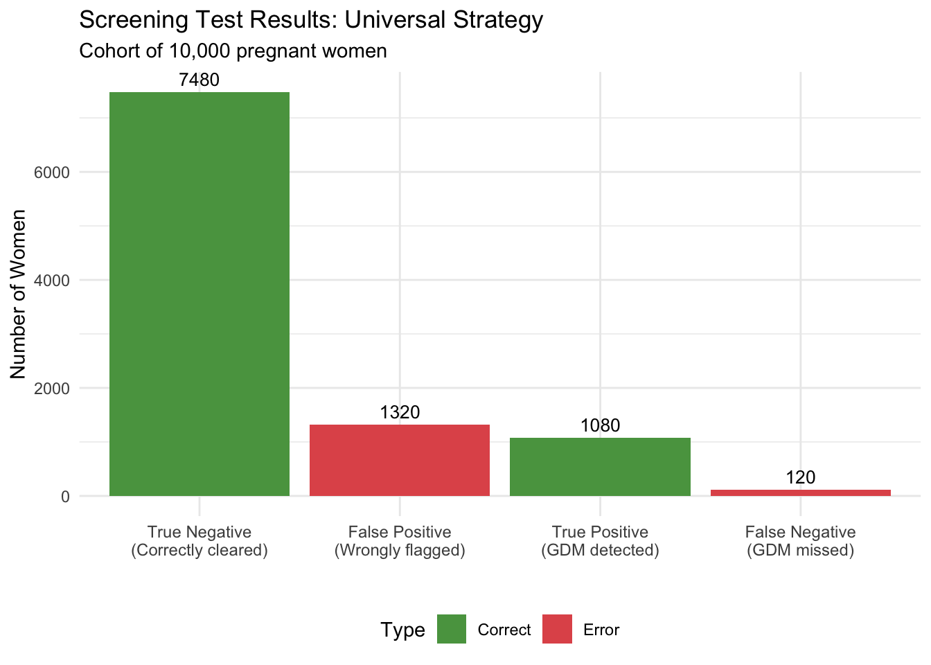
True negatives (correctly cleared): 7480

Code

library(ggplot2)

Warning: package 'ggplot2' was built under R version 4.5.2

Code

test_results <- data.frame(
  Category = c("True Positive\n(GDM detected)", "False Negative\n(GDM missed)",
                "False Positive\n(Wrongly flagged)", "True Negative\n(Correctly cleared)"),
  Count = c(true_positive, false_negative, false_positive, true_negative),
  Type = c("Correct", "Error", "Error", "Correct")
)

ggplot(test_results, aes(x = reorder(Category, -Count), y = Count, fill = Type)) +
  geom_col() +
  geom_text(aes(label = round(Count)), vjust = -0.5, size = 3.5) +
  scale_fill_manual(values = c("Correct" = "#59a14f", "Error" = "#e15759")) +
  labs(x = "", y = "Number of Women",
       title = "Screening Test Results: Universal Strategy",
       subtitle = paste0("Cohort of ", format(n_cohort, big.mark=","), " pregnant women")) +
  theme_minimal() +
  theme(legend.position = "bottom", axis.text.x = element_text(size = 9))

Figure 2: Distribution of screening test results — Universal Screening

Now let us calculate costs and outcomes:

Code

# --- Costs: Universal Screening ---

# Screening cost: everyone gets OGTT
cost_screening_universal <- n_cohort * cost_ogtt

# Treatment costs: true positives + false positives receive treatment
cost_treatment_universal <- (true_positive + false_positive) * cost_gdm_treatment

# Adverse outcome costs
# True positives: GDM treated → lower adverse probability
adverse_tp <- true_positive * p_adverse_gdm_treated
no_adverse_tp <- true_positive * (1 - p_adverse_gdm_treated)

# False negatives: GDM untreated → higher adverse probability
adverse_fn <- false_negative * p_adverse_gdm_untreated
no_adverse_fn <- false_negative * (1 - p_adverse_gdm_untreated)

# False positives: no GDM but treated → background adverse risk
adverse_fp <- false_positive * p_adverse_no_gdm
no_adverse_fp <- false_positive * (1 - p_adverse_no_gdm)

# True negatives: no GDM, correctly cleared → background risk
adverse_tn <- true_negative * p_adverse_no_gdm
no_adverse_tn <- true_negative * (1 - p_adverse_no_gdm)

# Total adverse outcomes and costs
total_adverse_universal <- adverse_tp + adverse_fn + adverse_fp + adverse_tn
total_no_adverse_universal <- no_adverse_tp + no_adverse_fn + no_adverse_fp + no_adverse_tn

cost_outcomes_universal <- total_adverse_universal * cost_adverse +
                           total_no_adverse_universal * cost_no_adverse

# Total cost
total_cost_universal <- cost_screening_universal + cost_treatment_universal +
                        cost_outcomes_universal

cat("=== Universal Screening: Cost Summary ===\n")

=== Universal Screening: Cost Summary ===

Code

cat("Screening cost: ₹", format(cost_screening_universal, big.mark = ","), "\n")

Screening cost: ₹ 2,500,000

Code

cat("Treatment cost: ₹", format(cost_treatment_universal, big.mark = ","), "\n")

Treatment cost: ₹ 19,200,000

Code

cat("Outcome costs: ₹", format(round(cost_outcomes_universal), big.mark = ","), "\n")

Outcome costs: ₹ 73,600,000

Code

cat("TOTAL COST: ₹", format(round(total_cost_universal), big.mark = ","), "\n")

TOTAL COST: ₹ 95,300,000

Code

cat("\nAdverse outcomes:", round(total_adverse_universal), "out of", n_cohort, "\n")


Adverse outcomes: 590 out of 10000

Code

# --- QALYs: Universal Screening ---

# QALYs by group
qaly_tp <- true_positive * ((1 - p_adverse_gdm_treated) * utility_gdm_treated +
           p_adverse_gdm_treated * utility_adverse)
qaly_fn <- false_negative * ((1 - p_adverse_gdm_untreated) * utility_no_adverse +
           p_adverse_gdm_untreated * utility_adverse)
qaly_fp <- false_positive * ((1 - p_adverse_no_gdm) * utility_gdm_treated +
           p_adverse_no_gdm * utility_adverse)
qaly_tn <- true_negative * ((1 - p_adverse_no_gdm) * utility_no_adverse +
           p_adverse_no_gdm * utility_adverse)

total_qaly_universal <- qaly_tp + qaly_fn + qaly_fp + qaly_tn

cat("Total QALYs (Universal Screening):", round(total_qaly_universal, 1), "\n")

Total QALYs (Universal Screening): 8674.4

Code

cat("Mean QALY per woman:", round(total_qaly_universal / n_cohort, 4), "\n")

Mean QALY per woman: 0.8674

Strategy 2: Risk-Based Screening

Only high-risk women are offered OGTT. Low-risk women are not screened.

Code

# --- Risk-Based Screening Strategy ---

n_high_risk <- n_cohort * prop_high_risk
n_low_risk  <- n_cohort * (1 - prop_high_risk)

# Among high-risk women
n_gdm_hr    <- n_high_risk * prev_gdm_high_risk
n_no_gdm_hr <- n_high_risk * (1 - prev_gdm_high_risk)

tp_hr <- n_gdm_hr * sens_ogtt
fn_hr <- n_gdm_hr * (1 - sens_ogtt)
fp_hr <- n_no_gdm_hr * (1 - spec_ogtt)
tn_hr <- n_no_gdm_hr * spec_ogtt

# Among low-risk women (NOT screened — GDM undetected)
n_gdm_lr    <- n_low_risk * prev_gdm_low_risk
n_no_gdm_lr <- n_low_risk * (1 - prev_gdm_low_risk)

cat("=== Risk-Based Screening Results ===\n")

=== Risk-Based Screening Results ===

Code

cat("High-risk women screened:", n_high_risk, "\n")

High-risk women screened: 6000

Code

cat("Low-risk women NOT screened:", n_low_risk, "\n")

Low-risk women NOT screened: 4000

Code

cat("GDM detected (high-risk true positives):", tp_hr, "\n")

GDM detected (high-risk true positives): 972

Code

cat("GDM missed in high-risk (false negatives):", fn_hr, "\n")

GDM missed in high-risk (false negatives): 108

Code

cat("GDM missed in low-risk (never screened):", n_gdm_lr, "\n")

GDM missed in low-risk (never screened): 120

Code

cat("Total GDM missed:", fn_hr + n_gdm_lr, "\n")

Total GDM missed: 228

Code

# --- Costs: Risk-Based Screening ---

# Screening cost: risk assessment for all, OGTT only for high-risk
cost_screening_risk <- n_cohort * cost_risk_assessment + n_high_risk * cost_ogtt

# Treatment cost: only high-risk true positives + false positives
cost_treatment_risk <- (tp_hr + fp_hr) * cost_gdm_treatment

# Adverse outcomes
# High-risk: detected GDM (treated)
adverse_tp_hr <- tp_hr * p_adverse_gdm_treated
# High-risk: missed GDM (untreated)
adverse_fn_hr <- fn_hr * p_adverse_gdm_untreated
# High-risk: false positives (background risk)
adverse_fp_hr <- fp_hr * p_adverse_no_gdm
# High-risk: true negatives
adverse_tn_hr <- tn_hr * p_adverse_no_gdm
# Low-risk: undetected GDM
adverse_gdm_lr <- n_gdm_lr * p_adverse_gdm_untreated
# Low-risk: no GDM
adverse_no_gdm_lr <- n_no_gdm_lr * p_adverse_no_gdm

total_adverse_risk <- adverse_tp_hr + adverse_fn_hr + adverse_fp_hr +
                      adverse_tn_hr + adverse_gdm_lr + adverse_no_gdm_lr

total_no_adverse_risk <- n_cohort - total_adverse_risk  # Simplified

cost_outcomes_risk <- total_adverse_risk * cost_adverse +
                      total_no_adverse_risk * cost_no_adverse

total_cost_risk <- cost_screening_risk + cost_treatment_risk + cost_outcomes_risk

cat("=== Risk-Based Screening: Cost Summary ===\n")

=== Risk-Based Screening: Cost Summary ===

Code

cat("Screening cost: ₹", format(cost_screening_risk, big.mark = ","), "\n")

Screening cost: ₹ 2e+06

Code

cat("Treatment cost: ₹", format(round(cost_treatment_risk), big.mark = ","), "\n")

Treatment cost: ₹ 13,680,000

Code

cat("Outcome costs: ₹", format(round(cost_outcomes_risk), big.mark = ","), "\n")

Outcome costs: ₹ 74,680,000

Code

cat("TOTAL COST: ₹", format(round(total_cost_risk), big.mark = ","), "\n")

TOTAL COST: ₹ 90,360,000

Code

cat("\nAdverse outcomes:", round(total_adverse_risk), "out of", n_cohort, "\n")


Adverse outcomes: 617 out of 10000

Code

# --- QALYs: Risk-Based Screening ---

qaly_tp_hr <- tp_hr * ((1 - p_adverse_gdm_treated) * utility_gdm_treated +
              p_adverse_gdm_treated * utility_adverse)
qaly_fn_hr <- fn_hr * ((1 - p_adverse_gdm_untreated) * utility_no_adverse +
              p_adverse_gdm_untreated * utility_adverse)
qaly_fp_hr <- fp_hr * ((1 - p_adverse_no_gdm) * utility_gdm_treated +
              p_adverse_no_gdm * utility_adverse)
qaly_tn_hr <- tn_hr * ((1 - p_adverse_no_gdm) * utility_no_adverse +
              p_adverse_no_gdm * utility_adverse)
qaly_gdm_lr <- n_gdm_lr * ((1 - p_adverse_gdm_untreated) * utility_no_adverse +
               p_adverse_gdm_untreated * utility_adverse)
qaly_no_gdm_lr <- n_no_gdm_lr * ((1 - p_adverse_no_gdm) * utility_no_adverse +
                  p_adverse_no_gdm * utility_adverse)

total_qaly_risk <- qaly_tp_hr + qaly_fn_hr + qaly_fp_hr +
                   qaly_tn_hr + qaly_gdm_lr + qaly_no_gdm_lr

cat("Total QALYs (Risk-Based Screening):", round(total_qaly_risk, 1), "\n")

Total QALYs (Risk-Based Screening): 8719.7

Code

cat("Mean QALY per woman:", round(total_qaly_risk / n_cohort, 4), "\n")

Mean QALY per woman: 0.872

Strategy 3: No Formal Screening

GDM is detected only when symptomatic (estimated detection rate ~25% based on clinical presentation alone).

Code

# --- No Screening Strategy ---

# Detection rate through clinical presentation alone
detection_rate_clinical <- 0.25

n_gdm_total <- n_cohort * prev_gdm
n_no_gdm_total <- n_cohort * (1 - prev_gdm)

n_gdm_detected_clinical <- n_gdm_total * detection_rate_clinical
n_gdm_undetected <- n_gdm_total * (1 - detection_rate_clinical)

# Costs: no screening cost, treatment only for clinically detected
cost_screening_none <- 0
cost_treatment_none <- n_gdm_detected_clinical * cost_gdm_treatment

# Adverse outcomes
adverse_detected <- n_gdm_detected_clinical * p_adverse_gdm_treated
adverse_undetected <- n_gdm_undetected * p_adverse_gdm_untreated
adverse_no_gdm_none <- n_no_gdm_total * p_adverse_no_gdm

total_adverse_none <- adverse_detected + adverse_undetected + adverse_no_gdm_none
total_no_adverse_none <- n_cohort - total_adverse_none

cost_outcomes_none <- total_adverse_none * cost_adverse +
                      total_no_adverse_none * cost_no_adverse

total_cost_none <- cost_screening_none + cost_treatment_none + cost_outcomes_none

# QALYs
qaly_detected <- n_gdm_detected_clinical * ((1 - p_adverse_gdm_treated) * utility_gdm_treated +
                 p_adverse_gdm_treated * utility_adverse)
qaly_undetected <- n_gdm_undetected * ((1 - p_adverse_gdm_untreated) * utility_no_adverse +
                   p_adverse_gdm_untreated * utility_adverse)
qaly_no_gdm_none <- n_no_gdm_total * ((1 - p_adverse_no_gdm) * utility_no_adverse +
                    p_adverse_no_gdm * utility_adverse)

total_qaly_none <- qaly_detected + qaly_undetected + qaly_no_gdm_none

cat("=== No Screening: Results ===\n")

=== No Screening: Results ===

Code

cat("GDM detected clinically:", n_gdm_detected_clinical, "out of", n_gdm_total, "\n")

GDM detected clinically: 300 out of 1200

Code

cat("TOTAL COST: ₹", format(round(total_cost_none), big.mark = ","), "\n")

TOTAL COST: ₹ 83,800,000

Code

cat("Adverse outcomes:", round(total_adverse_none), "out of", n_cohort, "\n")

Adverse outcomes: 785 out of 10000

Code

cat("Total QALYs:", round(total_qaly_none, 1), "\n")

Total QALYs: 8782.1

Comparing the Three Strategies

Code

# --- Summary Comparison ---
library(knitr)

results <- data.frame(
  Strategy = c("Universal Screening", "Risk-Based Screening", "No Screening"),
  Total_Cost = c(total_cost_universal, total_cost_risk, total_cost_none),
  Total_QALYs = c(total_qaly_universal, total_qaly_risk, total_qaly_none),
  Adverse_Outcomes = c(total_adverse_universal, total_adverse_risk, total_adverse_none)
)

# Format for display
results$Cost_per_Woman <- results$Total_Cost / n_cohort
results$QALY_per_Woman <- results$Total_QALYs / n_cohort
results$Adverse_Rate <- paste0(round(results$Adverse_Outcomes / n_cohort * 100, 1), "%")

results$Total_Cost <- paste0("₹", format(round(results$Total_Cost), big.mark = ","))

kable(results[, c("Strategy", "Total_Cost", "QALY_per_Woman", "Adverse_Rate")],
      col.names = c("Strategy", "Total Cost (cohort)", "QALY per Woman", "Adverse Outcome Rate"),
      digits = 4,
      caption = "Comparison of GDM Screening Strategies (cohort of 10,000 women)")

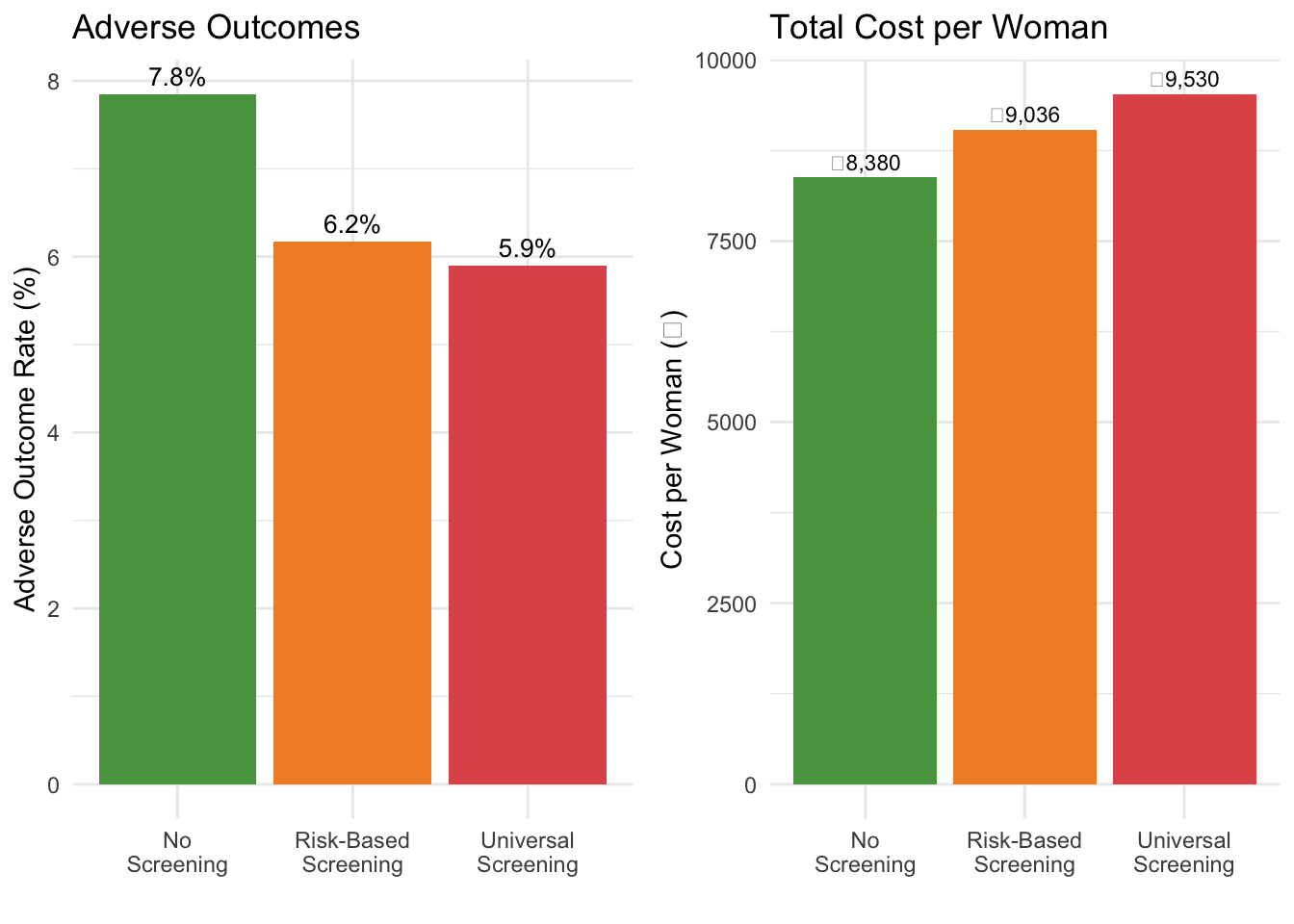
Comparison of GDM Screening Strategies (cohort of 10,000 women)
Strategy	Total Cost (cohort)	QALY per Woman	Adverse Outcome Rate
Universal Screening	₹95,300,000	0.8674	5.9%
Risk-Based Screening	₹90,360,000	0.8720	6.2%
No Screening	₹83,800,000	0.8782	7.8%

Code

adverse_data <- data.frame(
  Strategy = c("Universal\nScreening", "Risk-Based\nScreening", "No\nScreening"),
  Adverse_Rate = c(total_adverse_universal / n_cohort * 100,
                   total_adverse_risk / n_cohort * 100,
                   total_adverse_none / n_cohort * 100),
  Cost_Per_Woman = c(total_cost_universal / n_cohort,
                     total_cost_risk / n_cohort,
                     total_cost_none / n_cohort)
)

library(gridExtra)

p1 <- ggplot(adverse_data, aes(x = Strategy, y = Adverse_Rate, fill = Strategy)) +
  geom_col(show.legend = FALSE) +
  geom_text(aes(label = paste0(round(Adverse_Rate, 1), "%")), vjust = -0.5, size = 3.5) +
  scale_fill_manual(values = c("#59a14f", "#f28e2b", "#e15759")) +
  labs(x = "", y = "Adverse Outcome Rate (%)",
       title = "Adverse Outcomes") +
  theme_minimal()

p2 <- ggplot(adverse_data, aes(x = Strategy, y = Cost_Per_Woman, fill = Strategy)) +
  geom_col(show.legend = FALSE) +
  geom_text(aes(label = paste0("₹", format(round(Cost_Per_Woman), big.mark=","))), vjust = -0.5, size = 3) +
  scale_fill_manual(values = c("#59a14f", "#f28e2b", "#e15759")) +
  labs(x = "", y = "Cost per Woman (₹)",
       title = "Total Cost per Woman") +
  theme_minimal()

grid.arrange(p1, p2, ncol = 2)

Figure 3: Adverse outcome rates and costs across screening strategies

ICER and Net Monetary Benefit

Code

library(knitr)

# --- ICER Calculations ---
# Using no screening as the reference comparator

# Risk-based vs No screening
inc_cost_risk_vs_none <- total_cost_risk - total_cost_none
inc_qaly_risk_vs_none <- total_qaly_risk - total_qaly_none
icer_risk_vs_none <- inc_cost_risk_vs_none / inc_qaly_risk_vs_none

# Universal vs No screening
inc_cost_univ_vs_none <- total_cost_universal - total_cost_none
inc_qaly_univ_vs_none <- total_qaly_universal - total_qaly_none
icer_univ_vs_none <- inc_cost_univ_vs_none / inc_qaly_univ_vs_none

# Universal vs Risk-based
inc_cost_univ_vs_risk <- total_cost_universal - total_cost_risk
inc_qaly_univ_vs_risk <- total_qaly_universal - total_qaly_risk
icer_univ_vs_risk <- inc_cost_univ_vs_risk / inc_qaly_univ_vs_risk

# WTP threshold
wtp_india <- 170000

# --- 4-quadrant ICER interpretation ---
interpret_icer <- function(dc, dq, wtp) {
  if (dc < 0 & dq > 0) return("DOMINANT")
  if (dc > 0 & dq < 0) return("DOMINATED")
  if (dc > 0 & dq > 0) return(if (dc/dq < wtp) "Cost-effective" else "Not CE")
  return("Trade-off (cheaper but worse)")
}

# Summary table
kable(data.frame(
  Comparison = c("Risk-Based vs No Screening",
                 "Universal vs No Screening",
                 "Universal vs Risk-Based"),
  `Incr Cost/woman (₹)` = c(
    paste0("₹", format(round(inc_cost_risk_vs_none / n_cohort), big.mark = ",")),
    paste0("₹", format(round(inc_cost_univ_vs_none / n_cohort), big.mark = ",")),
    paste0("₹", format(round(inc_cost_univ_vs_risk / n_cohort), big.mark = ","))
  ),
  `Incr QALYs/woman` = c(
    round(inc_qaly_risk_vs_none / n_cohort, 4),
    round(inc_qaly_univ_vs_none / n_cohort, 4),
    round(inc_qaly_univ_vs_risk / n_cohort, 4)
  ),
  `ICER (₹/QALY)` = c(
    paste0("₹", format(round(icer_risk_vs_none), big.mark = ",")),
    paste0("₹", format(round(icer_univ_vs_none), big.mark = ",")),
    paste0("₹", format(round(icer_univ_vs_risk), big.mark = ","))
  ),
  Conclusion = c(
    interpret_icer(inc_cost_risk_vs_none, inc_qaly_risk_vs_none, wtp_india),
    interpret_icer(inc_cost_univ_vs_none, inc_qaly_univ_vs_none, wtp_india),
    interpret_icer(inc_cost_univ_vs_risk, inc_qaly_univ_vs_risk, wtp_india)
  ),
  check.names = FALSE
), align = "lrrrr",
   caption = paste0("Incremental cost-effectiveness (WTP = ₹", format(wtp_india, big.mark = ","), "/QALY)"))

Incremental cost-effectiveness (WTP = ₹170,000/QALY)
Comparison	Incr Cost/woman (₹)	Incr QALYs/woman	ICER (₹/QALY)	Conclusion
Risk-Based vs No Screening	₹656	-0.0062	₹-105,007	DOMINATED
Universal vs No Screening	₹1,150	-0.0108	₹-106,748	DOMINATED
Universal vs Risk-Based	₹494	-0.0045	₹-109,152	DOMINATED

Net Monetary Benefit

The ICER can be ambiguous when negative (DOMINANT and DOMINATED both produce negative ratios). The NMB gives an unambiguous answer: positive ΔNMB = adopt.

Code

# NMB = WTP × QALYs − Cost (per woman)
nmb_none <- wtp_india * (total_qaly_none / n_cohort) - (total_cost_none / n_cohort)
nmb_risk <- wtp_india * (total_qaly_risk / n_cohort) - (total_cost_risk / n_cohort)
nmb_univ <- wtp_india * (total_qaly_universal / n_cohort) - (total_cost_universal / n_cohort)

kable(data.frame(
  Strategy = c("No Screening", "Risk-Based Screening", "Universal Screening"),
  `NMB per woman (₹)` = c(
    paste0("₹", format(round(nmb_none), big.mark = ",")),
    paste0("₹", format(round(nmb_risk), big.mark = ",")),
    paste0("₹", format(round(nmb_univ), big.mark = ","))
  ),
  Ranking = rank(-c(nmb_none, nmb_risk, nmb_univ)),
  check.names = FALSE
), align = "lrr",
   caption = paste0("Net Monetary Benefit (WTP = ₹", format(wtp_india, big.mark = ","), "/QALY) — highest NMB is optimal"))

Net Monetary Benefit (WTP = ₹170,000/QALY) — highest NMB is optimal
Strategy	NMB per woman (₹)	Ranking
No Screening	₹140,917	1
Risk-Based Screening	₹139,199	2
Universal Screening	₹137,935	3

Reading the NMB Table

The strategy with the highest NMB is the optimal choice at the given WTP threshold. Unlike the ICER (which only compares pairs), NMB ranks all strategies simultaneously — making it easy to identify the best option when there are more than two comparators.

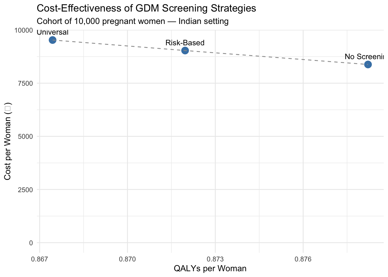
Visualising the Results

Code

library(ggplot2)

plot_data <- data.frame(
  Strategy = c("No Screening", "Risk-Based", "Universal"),
  Cost = c(total_cost_none / n_cohort,
           total_cost_risk / n_cohort,
           total_cost_universal / n_cohort),
  QALY = c(total_qaly_none / n_cohort,
           total_qaly_risk / n_cohort,
           total_qaly_universal / n_cohort)
)

ggplot(plot_data, aes(x = QALY, y = Cost, label = Strategy)) +
  geom_point(size = 4, colour = "steelblue") +
  geom_text(vjust = -1, hjust = 0.5, size = 3.5) +
  geom_line(linetype = "dashed", colour = "grey60") +
  labs(
    x = "QALYs per Woman",
    y = "Cost per Woman (₹)",
    title = "Cost-Effectiveness of GDM Screening Strategies",
    subtitle = "Cohort of 10,000 pregnant women — Indian setting"
  ) +
  theme_minimal() +
  expand_limits(y = 0)

Cost-effectiveness comparison of GDM screening strategies

What You Just Did

Without writing any code from scratch, you followed a complete diagnostic decision tree analysis:

Defined the clinical question using Indian epidemiological data
Structured the decision tree with three screening strategies
Populated it with parameters from published Indian literature
Calculated costs, QALYs, and ICERs for each strategy
Visualised the results on a cost-effectiveness plane

In Excel, changing a single parameter (say, GDM prevalence) would require tracing through multiple cells. In R, you change one number at the top and re-run the entire analysis.

Key References

Pujitha KS et al. (2024). National and regional prevalence of gestational diabetes mellitus in India: a systematic review and meta-analysis. BMC Public Health.
Seshiah V et al. (2008). Prevalence of gestational diabetes mellitus in South India. JAPI.
Mohan V et al. (2014). Comparison of screening for GDM using IADPSG, DIPSI, and WHO 1999 criteria.
Behboudi-Gandevani S et al. (2019). Worldwide prevalence of GDM: a systematic review.
HAPO Study Cooperative Research Group (2008). Hyperglycemia and Adverse Pregnancy Outcomes. NEJM.
NHM India. National Guidelines for Diagnosis & Management of Gestational Diabetes Mellitus.
Moss JR et al. (2007). Cost-effectiveness of screening for GDM. BJOG.

→ Next: Open gdm-exercise.qmd to practice modifying this model yourself.