Code
# Install if needed (uncomment once)
# install.packages("heemod")

library(heemod)
library(ggplot2)The same model rebuilt with a dedicated Markov modelling package
In the main Session 5, you built a CKD Markov model from scratch — writing matrix multiplication loops, half-cycle correction, and discounting by hand. That transparency is essential for understanding what a Markov model does.
But in practice, dedicated packages handle the mechanics for you and add built-in features for sensitivity analysis, plotting, and reporting. For Markov cohort models in R, heemod (Health Economic Evaluation MODelling) is the standard package. It was designed specifically for HTA and handles states, transitions, costs, utilities, discounting, half-cycle correction, DSA, and PSA out of the box.
This page rebuilds the identical CKD model using heemod, so you can see the same results produced by a different engine — and learn the package workflow you’d use in real projects.
# Install if needed (uncomment once)
# install.packages("heemod")
library(heemod)
library(ggplot2)In heemod, all model parameters go into a single define_parameters() call. This makes it easy to modify them later for sensitivity analysis — the package knows which values are inputs vs calculations.
param <- define_parameters(
  # --- Transition Probabilities: Standard Care ---
  p_12_std = 0.10,    # Early → Moderate
  p_1d     = 0.02,    # Early → Death (same both arms)
  p_23_std = 0.12,    # Moderate → Advanced
  p_2d     = 0.04,    # Moderate → Death (same both arms)
  p_3d     = 0.15,    # Advanced → Death (same both arms)

  # --- Treatment Effect ---
  hr = 0.66,           # Hazard ratio (ACE-inhibitor)
  p_12_int = 1 - (1 - p_12_std)^hr,
  p_23_int = 1 - (1 - p_23_std)^hr,

  # --- Costs (₹ per year) ---
  cost_early    = 12000,
  cost_moderate = 45000,
  cost_advanced = 350000,
  cost_ace      = 6000,
  cost_screen   = 500,

  # --- Utilities ---
  u_early    = 0.85,
  u_moderate = 0.72,
  u_advanced = 0.55,
  u_death    = 0.00,

  # --- Discount Rate ---
  dr = 0.03
)Parameters defined with define_parameters() can reference each other. The intervention transition probabilities (p_12_int, p_23_int) are computed from the standard care values and the hazard ratio — just like in the manual approach. If you change hr, both intervention probabilities update automatically.
Each health state gets its own define_state() call specifying the cost and utility per cycle. These are the state rewards — what accrues each year a patient spends in that state.
# --- States for STANDARD CARE ---
# discount() applies 3% annual discounting automatically using model_time
s_early_std <- define_state(
  cost = discount(cost_early, dr),
  utility = discount(u_early, dr)
)

s_moderate_std <- define_state(
  cost = discount(cost_moderate, dr),
  utility = discount(u_moderate, dr)
)

s_advanced_std <- define_state(
  cost = discount(cost_advanced, dr),
  utility = discount(u_advanced, dr)
)

s_death <- define_state(
  cost = 0,
  utility = discount(u_death, dr)
)

# --- States for INTERVENTION (ACE-inhibitor added to Early & Moderate) ---
# model_time == 1 adds the one-time screening cost only in the first cycle
# discount() wraps each cost/utility component for 3% annual discounting
s_early_int <- define_state(
  cost = discount(
    ifelse(model_time == 1, cost_screen, 0) + cost_early + cost_ace,
    dr
  ),
  utility = discount(u_early, dr)
)

s_moderate_int <- define_state(
  cost = discount(cost_moderate + cost_ace, dr),
  utility = discount(u_moderate, dr)
)

s_advanced_int <- define_state(
  cost = discount(cost_advanced, dr),   # ACE-inhibitor usually stopped in advanced CKD
  utility = discount(u_advanced, dr)
)define_transition() builds the matrix row-by-row. The special value C means “complement” — heemod automatically computes the diagonal (stay) probability so each row sums to 1.
# --- Standard Care ---
tm_std <- define_transition(
  state_names = c("EarlyCKD", "ModerateCKD", "AdvancedDialysis", "Death"),

  C,          p_12_std, 0,         p_1d,     # From Early
  0,          C,        p_23_std,  p_2d,     # From Moderate
  0,          0,        C,         p_3d,     # From Advanced
  0,          0,        0,         1         # Death (absorbing)
)

# --- Intervention ---
tm_int <- define_transition(
  state_names = c("EarlyCKD", "ModerateCKD", "AdvancedDialysis", "Death"),

  C,          p_12_int, 0,         p_1d,
  0,          C,        p_23_int,  p_2d,
  0,          0,        C,         p_3d,
  0,          0,        0,         1
)

cat("Standard Care Transition Matrix:\n")
Standard Care Transition Matrix:tm_stdA transition matrix, 4 states.
EarlyCKD ModerateCKD AdvancedDialysis Death
EarlyCKD C p_12_std p_1d
ModerateCKD C p_23_std p_2d
AdvancedDialysis C p_3d
Death 1 C Shorthand
The C (complement) value is heemod’s most convenient feature. Instead of manually typing 1 - p_12 - p_1d for the stay probability, you write C and the package handles the arithmetic. This eliminates a common source of bugs — forgetting to include all outgoing transitions when computing the “stay” probability.
A strategy combines a transition matrix with its state definitions. Each strategy represents one arm of the analysis.
strat_standard <- define_strategy(
  transition = tm_std,
  EarlyCKD         = s_early_std,
  ModerateCKD      = s_moderate_std,
  AdvancedDialysis = s_advanced_std,
  Death            = s_death
)

strat_intervention <- define_strategy(
  transition = tm_int,
  EarlyCKD         = s_early_int,
  ModerateCKD      = s_moderate_int,
  AdvancedDialysis = s_advanced_int,
  Death            = s_death
)run_model() simulates both strategies simultaneously. We specify 20 annual cycles, the cost and effect (utility) variable names, initial state distribution, and the correction method. In heemod, method = "life-table" applies half-cycle correction (averaging start and end of each cycle), equivalent to the manual (trace[t] + trace[t+1]) / 2 we used earlier. Note that discounting is handled via discount() inside define_state(), not in run_model() — this lets heemod apply the discount factor to each cycle’s values automatically using model_time.
res <- run_model(
  standard     = strat_standard,
  intervention = strat_intervention,
  parameters   = param,
  cycles       = 20,
  cost         = cost,
  effect       = utility,
  init         = c(10000, 0, 0, 0),
  method       = "life-table"
)

summary(res,
        threshold = 170000)
2 strategies run for 20 cycles.
Initial state counts:
EarlyCKD = 10000
ModerateCKD = 0
AdvancedDialysis = 0
Death = 0
Counting method: 'life-table'.
Values:
cost utility
standard 8065724874 84707.45
intervention 6473486025 92356.53
Net monetary benefit difference:
170000
standard 0.0
intervention 289258.2
Efficiency frontier:
intervention
Differences:
Cost Diff. Effect Diff. ICER Ref.
intervention -159223.9 0.7649076 -208160.9 standarddefine_state()
Two heemod features work together here. First, ifelse(model_time == 1, cost_screen, 0) adds the screening cost (₹500/person) only in cycle 1 — the same model_time / state_time trick works for any one-off cost (surgery, device implantation, initial diagnostics). Second, discount(value, dr) applies 3% annual discounting automatically using model_time — this replaces the manual discount factor vector. Both features are embedded in define_state(), keeping run_model() clean.
Let’s compare the heemod results with our manual implementation:
# Extract heemod results
heemod_summary <- summary(res)

cat("=== Cross-Validation ===\n\n")
=== Cross-Validation ===cat("Compare these heemod values with the manual R model and Excel:\n\n")Compare these heemod values with the manual R model and Excel:cat("If all three implementations agree (within rounding),\n")If all three implementations agree (within rounding),cat("the model is verified across independent platforms.\n\n")the model is verified across independent platforms.cat("The one-time screening cost is already included via\n")The one-time screening cost is already included viacat("model_time == 1 in the intervention's Early CKD state.\n")model_time == 1 in the intervention's Early CKD state.heemod provides built-in plotting for the Markov trace — the cohort distribution across states over time.
plot(res, type = "counts", panel = "by_strategy") +
  theme_minimal() +
  labs(title = "Markov Trace: CKD Progression Over 20 Years",
       subtitle = "Built-in heemod visualisation")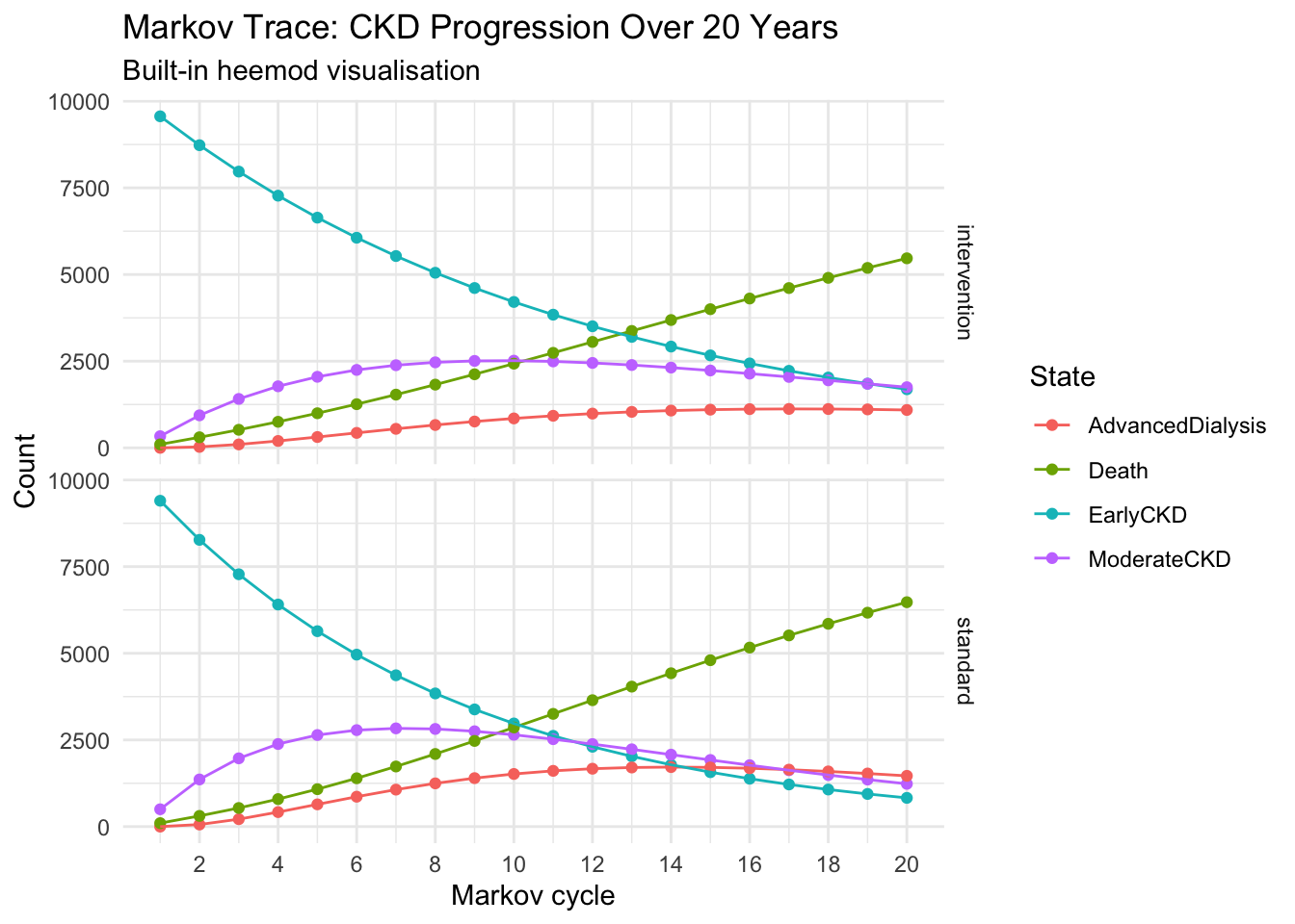
plot(res, type = "values", panel = "by_strategy") +
  theme_minimal()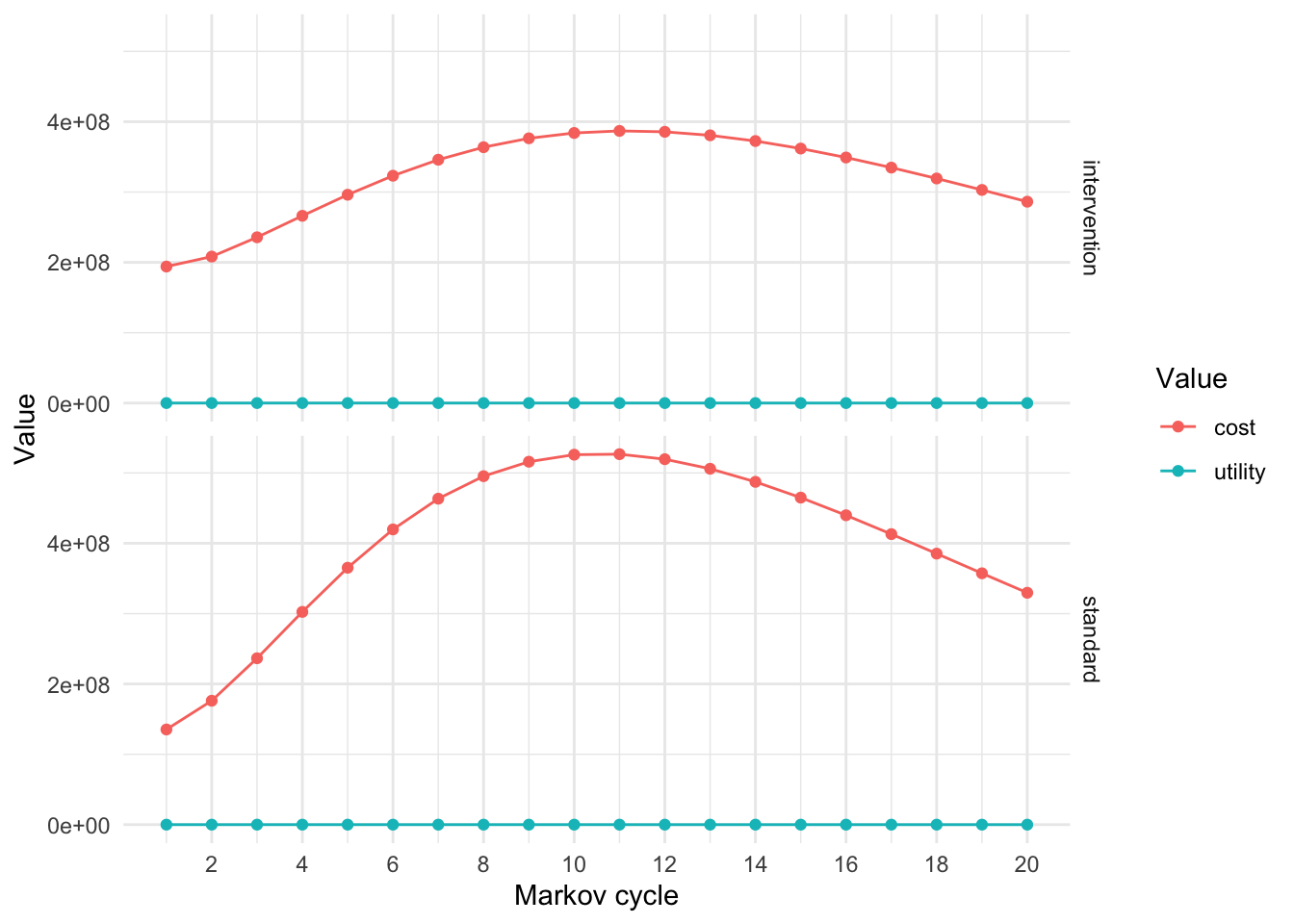
define_dsa() specifies which parameters to vary and their ranges. run_dsa() runs the model once per parameter at each extreme. The result is a tornado diagram showing which parameters drive the ICER most.
dsa_def <- define_dsa(
  p_12_std,      0.05,   0.15,     # Early→Moderate: ±50%
  p_23_std,      0.06,   0.18,     # Moderate→Advanced: ±50%
  p_3d,          0.10,   0.25,     # Advanced→Death: range
  hr,            0.50,   0.90,     # Treatment effect: wide range
  cost_early,    6000,   24000,    # ±100%
  cost_moderate, 25000,  75000,    # ±range
  cost_advanced, 150000, 600000,   # Public to private sector
  cost_ace,      3000,   12000,    # ±100%
  u_early,       0.75,   0.95,
  u_moderate,    0.60,   0.85,
  u_advanced,    0.40,   0.70,
  dr,            0.00,   0.05
)

res_dsa <- run_dsa(
  model   = res,
  dsa     = dsa_def
)
Running DSA on strategy 'standard'...Running DSA on strategy 'intervention'...plot(res_dsa,
result = "icer",
type = "difference")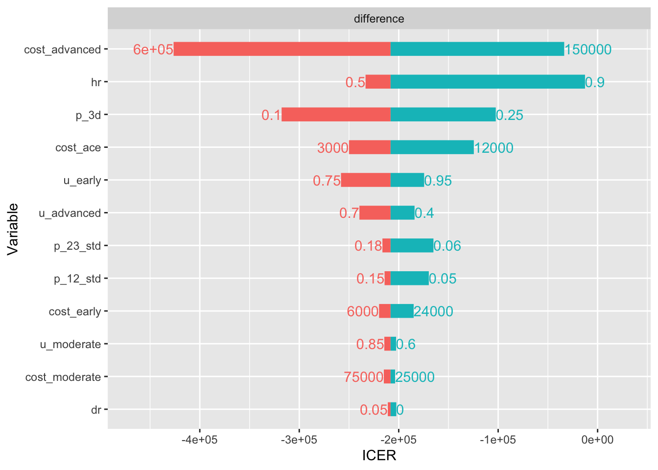
The parameter with the longest bar is the most influential on the ICER. If cost_advanced (dialysis cost) dominates, that confirms our manual one-way SA finding: the intervention’s value is driven primarily by how much dialysis costs it avoids.
PSA simultaneously varies all uncertain parameters across their distributions. define_psa() assigns a probability distribution to each parameter, and run_psa() draws 1,000 samples.
psa_def <- define_psa(
  # Transition probabilities: Beta distributions
  p_12_std ~ binomial(prob = 0.10, size = 100),
  p_23_std ~ binomial(prob = 0.12, size = 100),
  p_3d     ~ binomial(prob = 0.15, size = 100),
  p_1d     ~ binomial(prob = 0.02, size = 200),
  p_2d     ~ binomial(prob = 0.04, size = 200),

  # Treatment effect: Log-normal for hazard ratio
  hr ~ lognormal(meanlog = log(0.66), sdlog = 0.15),

  # Costs: Gamma distributions
  cost_early    ~ gamma(mean = 12000,  sd = 3000),
  cost_moderate ~ gamma(mean = 45000,  sd = 10000),
  cost_advanced ~ gamma(mean = 350000, sd = 70000),
  cost_ace      ~ gamma(mean = 6000,   sd = 1500),

  # Utilities: Beta-like via binomial
  u_early    ~ binomial(prob = 0.85, size = 100),
  u_moderate ~ binomial(prob = 0.72, size = 100),
  u_advanced ~ binomial(prob = 0.55, size = 100)
)

res_psa <- run_psa(
  model = res,
  psa   = psa_def,
  N     = 1000
)
Resampling strategy 'standard'...
Resampling strategy 'standard'...Resampling strategy 'intervention'...
Resampling strategy 'intervention'...The CE plane scatters all 1,000 PSA iterations on an incremental cost vs incremental QALY plot. Points in the south-east quadrant (lower cost, more QALYs) are dominant.
plot(res_psa, type = "ce") +
  theme_minimal() +
  labs(title = "Cost-Effectiveness Plane",
       subtitle = "Each dot = one PSA iteration")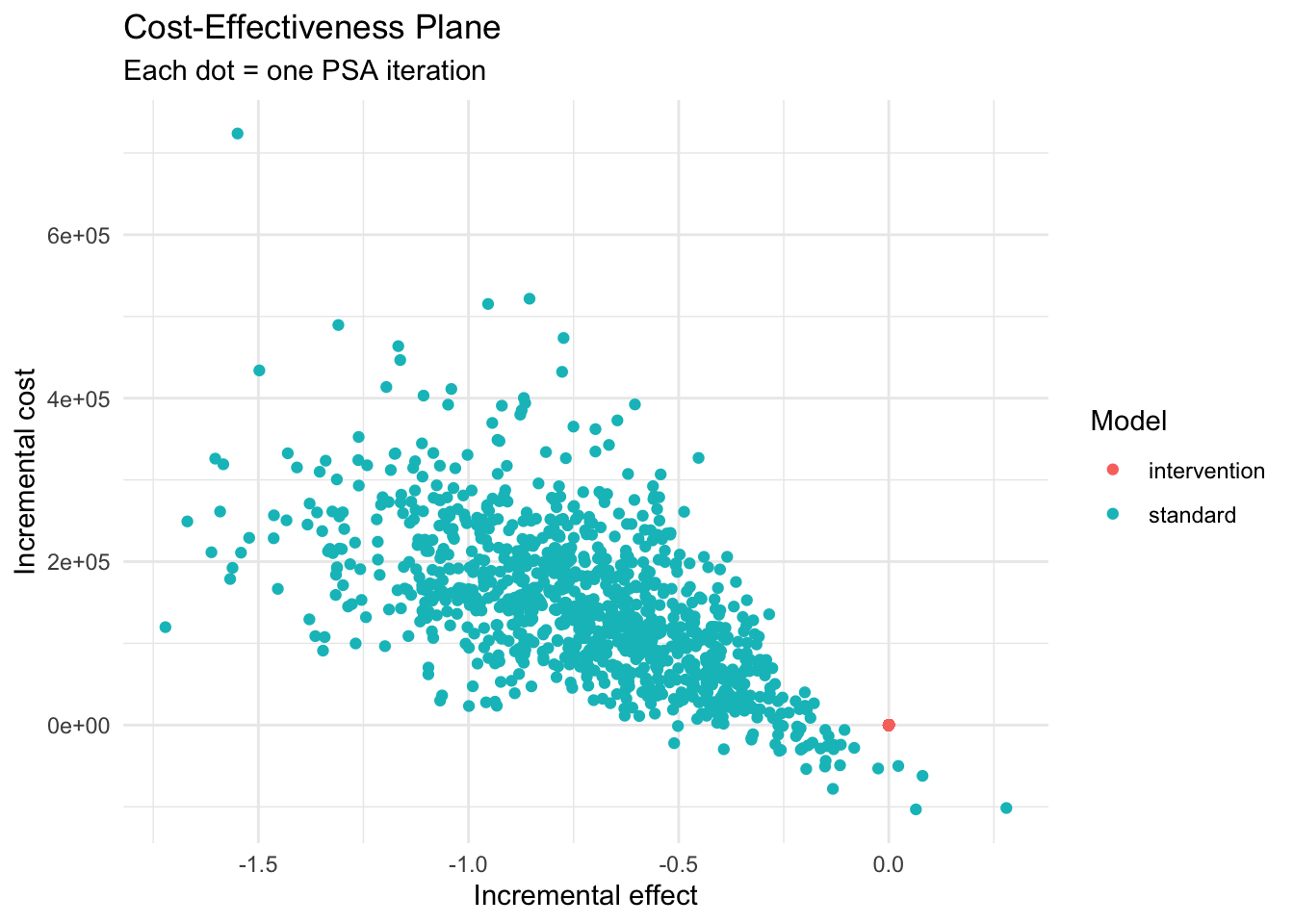
The CEAC shows the probability that each strategy is cost-effective across a range of WTP thresholds. At India’s threshold of ₹1,70,000/QALY, the intervention should have a high probability of being cost-effective.
plot(res_psa, type = "ac",
     max_wtp = 500000,
     log_scale = FALSE) +
  geom_vline(xintercept = 170000, linetype = "dashed", colour = "red") +
  annotate("text", x = 170000, y = 0.3, label = "WTP = ₹1,70,000\n(1× GDP/capita)",
           hjust = -0.1, colour = "red", size = 3) +
  theme_minimal() +
  labs(title = "Cost-Effectiveness Acceptability Curve",
       subtitle = "Probability of being cost-effective at each WTP threshold")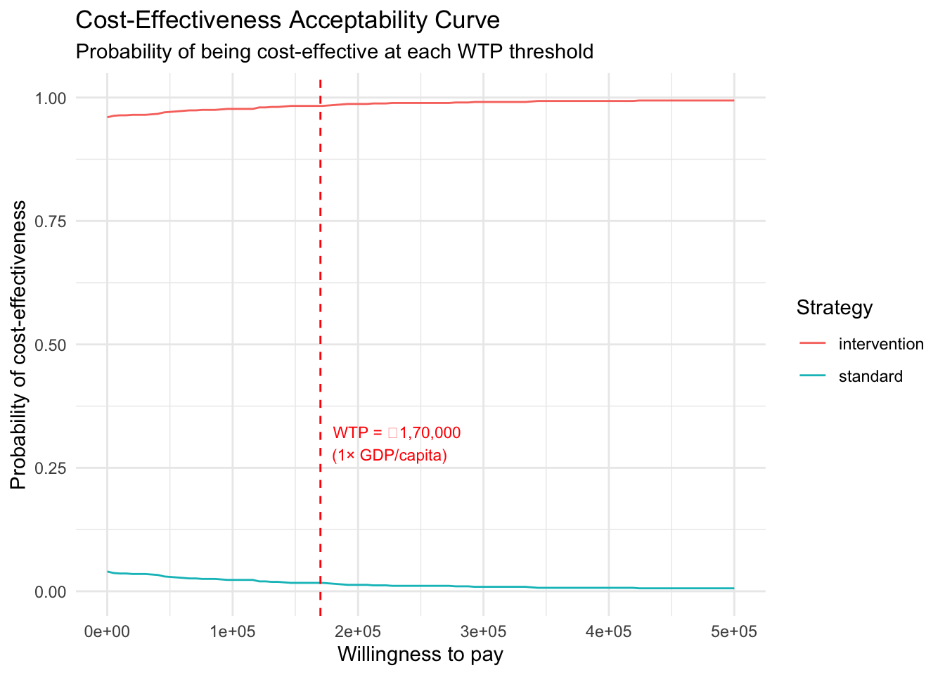
| Feature | Manual R | heemod |
|---|---|---|
| Transparency | Full — every calculation visible | Medium — internals hidden |
| Transition matrix | Manual matrix() construction |
define_transition() with C complement |
| Half-cycle correction | Manual averaging formula | Built-in method = "life-table" |
| Discounting | Manual discount factor vector | discount(value, rate) in define_state() |
| Markov trace plot | Manual ggplot code | plot(res, type = "counts") |
| One-way DSA | Manual loop over parameter values | define_dsa() + run_dsa() + tornado |
| PSA | Manual sampling + simulation loop | define_psa() + run_psa() |
| CE plane | Manual ggplot scatter | plot(res_psa, type = "ce") |
| CEAC | Manual NMB calculation + plot | plot(res_psa, type = "ac") |
| One-time costs | Manual addition outside the loop | ifelse(model_time == 1, cost, 0) in define_state() |
| Time-varying | Manual if statements in loop |
Built-in model_time, state_time |
| Learning value | High — teaches the mechanics | Lower — abstracts the mechanics |
| Production use | Error-prone at scale | Robust, tested, validated |
Use the manual approach when:
Use heemod when:
Best practice: Build both, cross-validate, then use heemod for the final analysis.
→ Back to: Session 5: CKD Markov Model (Manual) | Exercise