---
title: "Session 4 (Bonus): DES vs BMS Using the `rdecision` Package"
subtitle: "Same model, fewer lines — how dedicated HTA packages work"
format:
html:
toc: true
code-fold: show
code-tools: true
---
## Why This Tab Exists
In Session 4, we built the DES vs BMS decision tree **from scratch** — counting pathways, computing cost vectors, QALY vectors, and the ICER step by step. That was deliberate: you need to understand what happens inside the model before you let a package do it for you.
Now we rebuild the **exact same model** using [`rdecision`](https://cran.r-project.org/package=rdecision), a dedicated R package for decision-analytic modelling in health economics. The goal is to show:
1. **The results match** — same parameters, same ICER
2. **The code is shorter** — object-oriented tree construction replaces manual pathway arithmetic
3. **PSA is built in** — you can attach distributions and run Monte Carlo with one method call
4. **When to use which** — manual approach for learning and transparency; packages for production HTA
::: {.callout-note}
## Install first
If you haven't installed `rdecision`, run this once:
```r
install.packages("rdecision")
```
:::
## 1. How `rdecision` Thinks
The package uses an **object-oriented** (R6 class) approach. You build a decision tree from three types of objects:
| Object | What it represents | Analogy |
|--------|-------------------|---------|
| `DecisionNode` | The point where **we** choose (DES or BMS) | Square node in a tree diagram |
| `ChanceNode` | A point where **nature** decides (success/failure, restenosis/not) | Circle node |
| `LeafNode` | A terminal outcome (well, MI, death) — carries **utility** | Terminal box |
| `Action` | An edge from a decision node — carries a **cost** (e.g., stent cost) | Our choice |
| `Reaction` | An edge from a chance node — carries a **probability** and optional **cost** | Nature's outcome |
You connect these objects into a directed graph, hand it to `DecisionTree$new()`, and call `evaluate()`. The package automatically folds back the tree, computing expected costs and utilities per strategy.
::: {.callout-tip}
## Mental model
Think of it like assembling a circuit board. Each node is a component, each edge is a wire carrying probability and cost information. Once assembled, electricity (= patients) flows through the tree and the package tells you where they end up and what it costs.
:::
## 2. Parameters — Identical to Session 4
We use the **exact same inputs** so we can cross-validate the results.
```{r}
#| label: parameters
#| echo: true
library(rdecision)
library(knitr)

# ============================================================
# PARAMETERS — same as manual model (Session 4)
# ============================================================

# Cohort & framework
n_cohort      <- 1000
time_horizon  <- 5       # years
discount_rate <- 0.03
discount_factor <- sum(1 / (1 + discount_rate)^(0:(time_horizon - 1)))

# --- Probabilities ---
p_success_des <- 0.97
p_success_bms <- 0.96

p_restenosis_des <- 0.08
p_restenosis_bms <- 0.20

p_mace_des_no_restenosis <- 0.08
p_mace_bms_no_restenosis <- 0.15

p_mace_des_restenosis <- 0.15
p_mace_bms_restenosis <- 0.25

p_mi_given_mace        <- 0.70
p_cardiac_death_given_mace <- 0.30

p_cabg_if_restenosis <- 0.20

# --- Costs (₹) ---
cost_des_stent <- 38933
cost_bms_stent <- 10693
cost_procedure <- 120000
cost_dapt_des_annual <- 8000
cost_dapt_bms_annual <- 3000
cost_followup_annual <- 5000
cost_repeat_pci <- 180000
cost_cabg       <- 250000
cost_mi_management <- 200000
cost_cardiac_death_cost <- 50000

# --- Utilities ---
u_well  <- 0.85
u_rest  <- 0.78
u_mi    <- 0.65
u_death <- 0.00
```
::: {.callout-important}
## Same numbers, different approach
Every single parameter above is identical to Session 4. The only difference is *how we feed them into the model*. This lets us verify that the package gives the same answer.
:::
## 3. Pre-computing Composite Costs and Utilities
`rdecision` assigns costs to **edges** and utilities to **leaf nodes**. Our model has composite costs (e.g., initial PCI + stent + medications over 5 years) that we need to pre-compute so they can be attached to the right edges and leaves.
```{r}
#| label: composite-costs
#| echo: true
# ============================================================
# COMPOSITE COSTS FOR EDGES
# ============================================================

# Medication costs (discounted over time horizon) — differs by arm
med_cost_des <- cost_dapt_des_annual + cost_followup_annual * discount_factor
med_cost_bms <- cost_dapt_bms_annual + cost_followup_annual * discount_factor

# Initial PCI + stent + medications (per patient, successful PCI)
edge_cost_des <- cost_procedure + cost_des_stent + med_cost_des
edge_cost_bms <- cost_procedure + cost_bms_stent + med_cost_bms

# Procedural failure → CABG cost + medications
edge_cost_failure_des <- cost_cabg + med_cost_des
edge_cost_failure_bms <- cost_cabg + med_cost_bms

# Restenosis management (weighted: 80% repeat PCI, 20% CABG)
cost_restenosis_mgmt <- (1 - p_cabg_if_restenosis) * cost_repeat_pci +
                         p_cabg_if_restenosis * cost_cabg

# MACE costs at leaf level (weighted by MI vs death split)
# We'll handle MI/death split via separate branches
```
## 4. Composite Utilities for Leaf Nodes
In `rdecision`, leaf node utility must be a **weight between 0 and 1** — it represents the average quality of life in that health state. The package then multiplies this weight by the `interval` (time spent in state) to compute QALYs. So we need two things per leaf: an **average utility weight** and an **interval**.
Since our patients have different health trajectories (e.g., well for 2 years then MI), we compute the **time-weighted average utility** for each terminal state and set the interval to our 5-year horizon.
```{r}
#| label: composite-utilities
#| echo: true
# ============================================================
# LEAF UTILITIES — average utility weight (must be ≤ 1)
# rdecision computes QALY = utility × interval (in years)
# So we use time-weighted average utility over the horizon
# ============================================================

# Interval for all leaves: 5 years (expressed as difftime)
leaf_interval <- as.difftime(time_horizon * 365.25, units = "days")

# Well (no restenosis, no MACE) — full 5 years at u_well
leaf_u_well <- u_well   # 0.85

# Restenosis but recovered (no MACE after repeat intervention)
# 6 months unwell pre-intervention, then recovered for 4.5 years
# Average: (0.85 × 0.5 + 0.78 × 4.5) / 5
leaf_u_rest_ok <- (u_well * 0.5 + u_rest * (time_horizon - 0.5)) / time_horizon

# MI survivor — ~2 years well before MI, then reduced utility
# Average: (0.85 × 2 + 0.65 × 3) / 5
leaf_u_mi <- (u_well * 2 + u_mi * (time_horizon - 2)) / time_horizon

# Cardiac death — well until midpoint, then dead (utility 0)
# Average: (0.85 × 2.5 + 0 × 2.5) / 5
leaf_u_death <- (u_well * (time_horizon / 2)) / time_horizon

# Procedural failure → CABG → recovery (restenosis-like recovery)
leaf_u_failure <- u_rest   # 0.78
```
::: {.callout-note}
## Why average utility?
`rdecision` uses `QALY = utility × interval`. Our manual model computed total QALYs directly (e.g., `0.85 × 2 + 0.65 × 3 = 3.65`). The package achieves the same by: average utility `= 3.65 / 5 = 0.73`, interval = 5 years, so `0.73 × 5 = 3.65 QALYs`. Same result, different route.
:::
## 5. Building the Tree — Node by Node
This is where `rdecision` shines. We define nodes, connect them with edges, and the package handles the rollback arithmetic.
```{r}
#| label: build-tree
#| echo: true
# ============================================================
# STEP 1: CREATE ALL NODES
# ============================================================

# --- Decision node (root) ---
d_stent <- DecisionNode$new("PCI Stent Choice")

# --- DES arm: chance nodes ---
c_des_proc     <- ChanceNode$new("DES: Procedure")
c_des_rest     <- ChanceNode$new("DES: Restenosis?")
c_des_mace_r   <- ChanceNode$new("DES: MACE (post-restenosis)")
c_des_mace_nr  <- ChanceNode$new("DES: MACE (no restenosis)")
c_des_mace_type_r  <- ChanceNode$new("DES: MACE type (restenosis)")
c_des_mace_type_nr <- ChanceNode$new("DES: MACE type (no restenosis)")

# --- DES arm: leaf nodes (terminal outcomes with utility + interval) ---
l_des_failure     <- LeafNode$new("DES: Failure→CABG",        utility = leaf_u_failure,  interval = leaf_interval)
l_des_rest_well   <- LeafNode$new("DES: Restenosis→Well",     utility = leaf_u_rest_ok,  interval = leaf_interval)
l_des_rest_mi     <- LeafNode$new("DES: Restenosis→MI",       utility = leaf_u_mi,       interval = leaf_interval)
l_des_rest_death  <- LeafNode$new("DES: Restenosis→Death",    utility = leaf_u_death,    interval = leaf_interval)
l_des_norest_well <- LeafNode$new("DES: No Rest→Well",        utility = leaf_u_well,     interval = leaf_interval)
l_des_norest_mi   <- LeafNode$new("DES: No Rest→MI",          utility = leaf_u_mi,       interval = leaf_interval)
l_des_norest_death <- LeafNode$new("DES: No Rest→Death",      utility = leaf_u_death,    interval = leaf_interval)

# --- BMS arm: chance nodes ---
c_bms_proc     <- ChanceNode$new("BMS: Procedure")
c_bms_rest     <- ChanceNode$new("BMS: Restenosis?")
c_bms_mace_r   <- ChanceNode$new("BMS: MACE (post-restenosis)")
c_bms_mace_nr  <- ChanceNode$new("BMS: MACE (no restenosis)")
c_bms_mace_type_r  <- ChanceNode$new("BMS: MACE type (restenosis)")
c_bms_mace_type_nr <- ChanceNode$new("BMS: MACE type (no restenosis)")

# --- BMS arm: leaf nodes ---
l_bms_failure     <- LeafNode$new("BMS: Failure→CABG",        utility = leaf_u_failure,  interval = leaf_interval)
l_bms_rest_well   <- LeafNode$new("BMS: Restenosis→Well",     utility = leaf_u_rest_ok,  interval = leaf_interval)
l_bms_rest_mi     <- LeafNode$new("BMS: Restenosis→MI",       utility = leaf_u_mi,       interval = leaf_interval)
l_bms_rest_death  <- LeafNode$new("BMS: Restenosis→Death",    utility = leaf_u_death,    interval = leaf_interval)
l_bms_norest_well <- LeafNode$new("BMS: No Rest→Well",        utility = leaf_u_well,     interval = leaf_interval)
l_bms_norest_mi   <- LeafNode$new("BMS: No Rest→MI",          utility = leaf_u_mi,       interval = leaf_interval)
l_bms_norest_death <- LeafNode$new("BMS: No Rest→Death",      utility = leaf_u_death,    interval = leaf_interval)
```
::: {.callout-note}
## Why so many nodes?
In the manual model, we handled MI vs cardiac death with a simple multiplication (`total_mace * 0.70` for MI). In `rdecision`, every branch must be an explicit node-edge pair. This is more verbose but also more transparent — the tree diagram shows *every* possible pathway.
:::
## 6. Wiring the Edges — Actions and Reactions
```{r}
#| label: build-edges
#| echo: true
# ============================================================
# STEP 2: CREATE ALL EDGES
# ============================================================

# --- Decision → DES or BMS (Actions carry the stent choice cost) ---
a_des <- Action$new(d_stent, c_des_proc, cost = 0, label = "DES")
a_bms <- Action$new(d_stent, c_bms_proc, cost = 0, label = "BMS")

# ================================================================
# DES ARM EDGES
# ================================================================

# Procedure success/failure
r_des_success <- Reaction$new(c_des_proc, c_des_rest,
                               p = p_success_des,
                               cost = edge_cost_des,
                               label = "Success")
r_des_failure <- Reaction$new(c_des_proc, l_des_failure,
                               p = NA_real_,
                               cost = edge_cost_failure_des,
                               label = "Failure→CABG")

# Restenosis or not (among successes)
r_des_rest    <- Reaction$new(c_des_rest, c_des_mace_r,
                               p = p_restenosis_des,
                               cost = cost_restenosis_mgmt,
                               label = "Restenosis")
r_des_norest  <- Reaction$new(c_des_rest, c_des_mace_nr,
                               p = NA_real_,
                               cost = 0,
                               label = "No Restenosis")

# MACE among restenosis patients
r_des_mace_r_yes <- Reaction$new(c_des_mace_r, c_des_mace_type_r,
                                  p = p_mace_des_restenosis,
                                  cost = 0,
                                  label = "MACE")
r_des_mace_r_no  <- Reaction$new(c_des_mace_r, l_des_rest_well,
                                  p = NA_real_,
                                  cost = 0,
                                  label = "No MACE")

# MACE type split (restenosis pathway)
r_des_rest_mi    <- Reaction$new(c_des_mace_type_r, l_des_rest_mi,
                                  p = p_mi_given_mace,
                                  cost = cost_mi_management,
                                  label = "MI")
r_des_rest_death <- Reaction$new(c_des_mace_type_r, l_des_rest_death,
                                  p = NA_real_,
                                  cost = cost_cardiac_death_cost,
                                  label = "Cardiac Death")

# MACE among no-restenosis patients
r_des_mace_nr_yes <- Reaction$new(c_des_mace_nr, c_des_mace_type_nr,
                                   p = p_mace_des_no_restenosis,
                                   cost = 0,
                                   label = "MACE")
r_des_mace_nr_no  <- Reaction$new(c_des_mace_nr, l_des_norest_well,
                                   p = NA_real_,
                                   cost = 0,
                                   label = "No MACE")

# MACE type split (no-restenosis pathway)
r_des_norest_mi    <- Reaction$new(c_des_mace_type_nr, l_des_norest_mi,
                                    p = p_mi_given_mace,
                                    cost = cost_mi_management,
                                    label = "MI")
r_des_norest_death <- Reaction$new(c_des_mace_type_nr, l_des_norest_death,
                                    p = NA_real_,
                                    cost = cost_cardiac_death_cost,
                                    label = "Cardiac Death")

# ================================================================
# BMS ARM EDGES (same structure, different probabilities and costs)
# ================================================================

r_bms_success <- Reaction$new(c_bms_proc, c_bms_rest,
                               p = p_success_bms,
                               cost = edge_cost_bms,
                               label = "Success")
r_bms_failure <- Reaction$new(c_bms_proc, l_bms_failure,
                               p = NA_real_,
                               cost = edge_cost_failure_bms,
                               label = "Failure→CABG")

r_bms_rest    <- Reaction$new(c_bms_rest, c_bms_mace_r,
                               p = p_restenosis_bms,
                               cost = cost_restenosis_mgmt,
                               label = "Restenosis")
r_bms_norest  <- Reaction$new(c_bms_rest, c_bms_mace_nr,
                               p = NA_real_,
                               cost = 0,
                               label = "No Restenosis")

r_bms_mace_r_yes <- Reaction$new(c_bms_mace_r, c_bms_mace_type_r,
                                  p = p_mace_bms_restenosis,
                                  cost = 0,
                                  label = "MACE")
r_bms_mace_r_no  <- Reaction$new(c_bms_mace_r, l_bms_rest_well,
                                  p = NA_real_,
                                  cost = 0,
                                  label = "No MACE")

r_bms_rest_mi    <- Reaction$new(c_bms_mace_type_r, l_bms_rest_mi,
                                  p = p_mi_given_mace,
                                  cost = cost_mi_management,
                                  label = "MI")
r_bms_rest_death <- Reaction$new(c_bms_mace_type_r, l_bms_rest_death,
                                  p = NA_real_,
                                  cost = cost_cardiac_death_cost,
                                  label = "Cardiac Death")

r_bms_mace_nr_yes <- Reaction$new(c_bms_mace_nr, c_bms_mace_type_nr,
                                   p = p_mace_bms_no_restenosis,
                                   cost = 0,
                                   label = "MACE")
r_bms_mace_nr_no  <- Reaction$new(c_bms_mace_nr, l_bms_norest_well,
                                   p = NA_real_,
                                   cost = 0,
                                   label = "No MACE")

r_bms_norest_mi    <- Reaction$new(c_bms_mace_type_nr, l_bms_norest_mi,
                                    p = p_mi_given_mace,
                                    cost = cost_mi_management,
                                    label = "MI")
r_bms_norest_death <- Reaction$new(c_bms_mace_type_nr, l_bms_norest_death,
                                    p = NA_real_,
                                    cost = cost_cardiac_death_cost,
                                    label = "Cardiac Death")
```
::: {.callout-tip}
## The `p = NA_real_` trick
When a chance node has two outcomes, you only need to specify the probability for one. Setting the other to `NA_real_` tells `rdecision` to compute the complement automatically (so they sum to 1). This avoids errors from probabilities not adding up.
:::
## 7. Assemble and Evaluate the Tree
Now we hand all nodes and edges to `DecisionTree$new()` and call `evaluate()`.
```{r}
#| label: assemble-evaluate
#| echo: true
# ============================================================
# STEP 3: BUILD THE DECISION TREE
# ============================================================

# Collect all nodes
V <- list(
  d_stent,
  # DES nodes
  c_des_proc, c_des_rest,
  c_des_mace_r, c_des_mace_nr,
  c_des_mace_type_r, c_des_mace_type_nr,
  l_des_failure, l_des_rest_well, l_des_rest_mi, l_des_rest_death,
  l_des_norest_well, l_des_norest_mi, l_des_norest_death,
  # BMS nodes
  c_bms_proc, c_bms_rest,
  c_bms_mace_r, c_bms_mace_nr,
  c_bms_mace_type_r, c_bms_mace_type_nr,
  l_bms_failure, l_bms_rest_well, l_bms_rest_mi, l_bms_rest_death,
  l_bms_norest_well, l_bms_norest_mi, l_bms_norest_death
)

# Collect all edges
E <- list(
  a_des, a_bms,
  # DES edges
  r_des_success, r_des_failure,
  r_des_rest, r_des_norest,
  r_des_mace_r_yes, r_des_mace_r_no,
  r_des_rest_mi, r_des_rest_death,
  r_des_mace_nr_yes, r_des_mace_nr_no,
  r_des_norest_mi, r_des_norest_death,
  # BMS edges
  r_bms_success, r_bms_failure,
  r_bms_rest, r_bms_norest,
  r_bms_mace_r_yes, r_bms_mace_r_no,
  r_bms_rest_mi, r_bms_rest_death,
  r_bms_mace_nr_yes, r_bms_mace_nr_no,
  r_bms_norest_mi, r_bms_norest_death
)

# Build the tree
dt <- DecisionTree$new(V, E)

# ============================================================
# STEP 4: EVALUATE — one line does all the rollback!
# ============================================================
results <- dt$evaluate()

kable(results,
      caption = "rdecision output: expected per-patient cost and utility by strategy",
      digits = 2)
```
::: {.callout-important}
## One line replaces 80 lines
The `dt$evaluate()` call replaces all of Sections 6–9 from the manual model. It traces every pathway, weights by probability, accumulates costs along edges, and accumulates utilities at leaves — automatically.
:::
## 8. Cross-Validation — Does It Match?
Let's compare the `rdecision` output against our manual calculation.
The `evaluate()` output is a **long-format** data frame — one row per strategy, identified by the `PCI.Stent.Choice` column (named after our decision node). Let's look at it and then compare with the manual model:
```{r}
#| label: cross-validate
#| echo: true
# ============================================================
# EXTRACT rdecision RESULTS
# ============================================================
# evaluate() returns long format: 2 rows × 7 cols
# Columns: Run, PCI.Stent.Choice, Probability, Cost, Benefit, Utility, QALY

des_row <- results[results$PCI.Stent.Choice == "DES", ]
bms_row <- results[results$PCI.Stent.Choice == "BMS", ]

cost_des_pkg <- des_row$Cost
cost_bms_pkg <- bms_row$Cost
qaly_des_pkg <- des_row$QALY
qaly_bms_pkg <- bms_row$QALY

icer_pkg <- (cost_des_pkg - cost_bms_pkg) / (qaly_des_pkg - qaly_bms_pkg)

# ============================================================
# MANUAL MODEL (compact version from Session 4 run_model)
# ============================================================

des_s   <- n_cohort * p_success_des
des_r   <- des_s * p_restenosis_des
des_nr  <- des_s * (1 - p_restenosis_des)
des_mac <- des_r * p_mace_des_restenosis + des_nr * p_mace_des_no_restenosis
des_m   <- des_mac * p_mi_given_mace
des_d   <- des_mac * p_cardiac_death_given_mace

bms_s   <- n_cohort * p_success_bms
bms_r   <- bms_s * p_restenosis_bms
bms_nr  <- bms_s * (1 - p_restenosis_bms)
bms_mac <- bms_r * p_mace_bms_restenosis + bms_nr * p_mace_bms_no_restenosis
bms_m   <- bms_mac * p_mi_given_mace
bms_d   <- bms_mac * p_cardiac_death_given_mace

tc_des <- des_s * (cost_procedure + cost_des_stent) +
          (n_cohort - des_s) * cost_cabg +
          n_cohort * cost_dapt_des_annual +
          n_cohort * cost_followup_annual * discount_factor +
          des_r * cost_restenosis_mgmt +
          des_m * cost_mi_management + des_d * cost_cardiac_death_cost

tc_bms <- bms_s * (cost_procedure + cost_bms_stent) +
          (n_cohort - bms_s) * cost_cabg +
          n_cohort * cost_dapt_bms_annual +
          n_cohort * cost_followup_annual * discount_factor +
          bms_r * cost_restenosis_mgmt +
          bms_m * cost_mi_management + bms_d * cost_cardiac_death_cost

tq_des <- (des_nr - des_nr * p_mace_des_no_restenosis) * u_well * time_horizon +
          (des_r - des_r * p_mace_des_restenosis) * (u_well * 0.5 + u_rest * (time_horizon - 0.5)) +
          des_m * (u_well * 2 + u_mi * 3) +
          des_d * u_well * (time_horizon / 2) +
          (n_cohort - des_s) * u_rest * time_horizon

tq_bms <- (bms_nr - bms_nr * p_mace_bms_no_restenosis) * u_well * time_horizon +
          (bms_r - bms_r * p_mace_bms_restenosis) * (u_well * 0.5 + u_rest * (time_horizon - 0.5)) +
          bms_m * (u_well * 2 + u_mi * 3) +
          bms_d * u_well * (time_horizon / 2) +
          (n_cohort - bms_s) * u_rest * time_horizon

icer_manual <- (tc_des - tc_bms) / (tq_des - tq_bms)

# ============================================================
# COMPARISON TABLE
# ============================================================
fmt <- function(x) paste0("₹", format(round(x), big.mark = ","))

comparison <- data.frame(
  Metric = c("Cost per patient (DES)",
             "Cost per patient (BMS)",
             "QALYs per patient (DES)",
             "QALYs per patient (BMS)",
             "ICER (₹/QALY)"),
  Manual = c(fmt(tc_des / n_cohort),
             fmt(tc_bms / n_cohort),
             round(tq_des / n_cohort, 4),
             round(tq_bms / n_cohort, 4),
             fmt(icer_manual)),
  rdecision = c(fmt(cost_des_pkg),
                fmt(cost_bms_pkg),
                round(qaly_des_pkg, 4),
                round(qaly_bms_pkg, 4),
                fmt(icer_pkg))
)

kable(comparison, col.names = c("Metric", "Manual (Session 4)", "rdecision Package"),
      caption = "Cross-validation: Manual vs rdecision results",
      align = c("l", "r", "r"))
```
::: {.callout-warning}
## Small differences are expected
The manual model and `rdecision` may show minor rounding differences (a few rupees). This is normal — the approaches compute the same expected values but through different arithmetic paths. What matters is that the ICER and the qualitative conclusion (dominant, cost-effective, or not) are the same.
:::
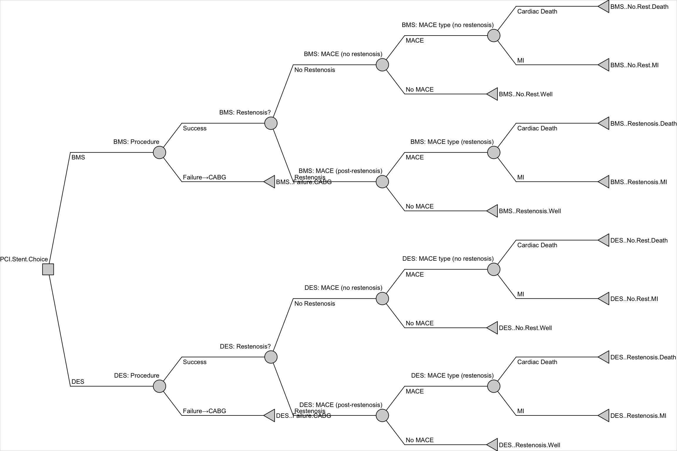
## 9. Built-in Feature: Drawing the Decision Tree
One advantage of `rdecision` is that the tree structure is stored as a formal graph object. The package provides a `draw()` method to visualise it directly — no need for separate `DiagrammeR` code.
```{r}
#| label: fig-draw-tree
#| echo: true
#| fig-cap: "Decision tree drawn by rdecision's built-in draw() method"
#| fig-width: 12
#| fig-height: 8
# rdecision can draw the tree it built — one line!
dt$draw(border = TRUE)
```
::: {.callout-tip}
## Model and diagram stay in sync
When you build the tree manually with `DiagrammeR::grViz()` (as in Session 4), the diagram is separate from the model — you could accidentally make the diagram show different probabilities than the code uses. With `rdecision`, the diagram *is* the model. Change a probability and the diagram updates automatically.
:::
The package also exports to **GraphViz DOT notation** for publication-quality figures:
```{r}
#| label: dot-export
#| echo: true
# Export tree to DOT format (for GraphViz rendering or LaTeX)
dot_code <- dt$as_DOT(rankdir = "LR")
cat(substr(dot_code, 1, 500), "...\n")  # show first 500 chars
```
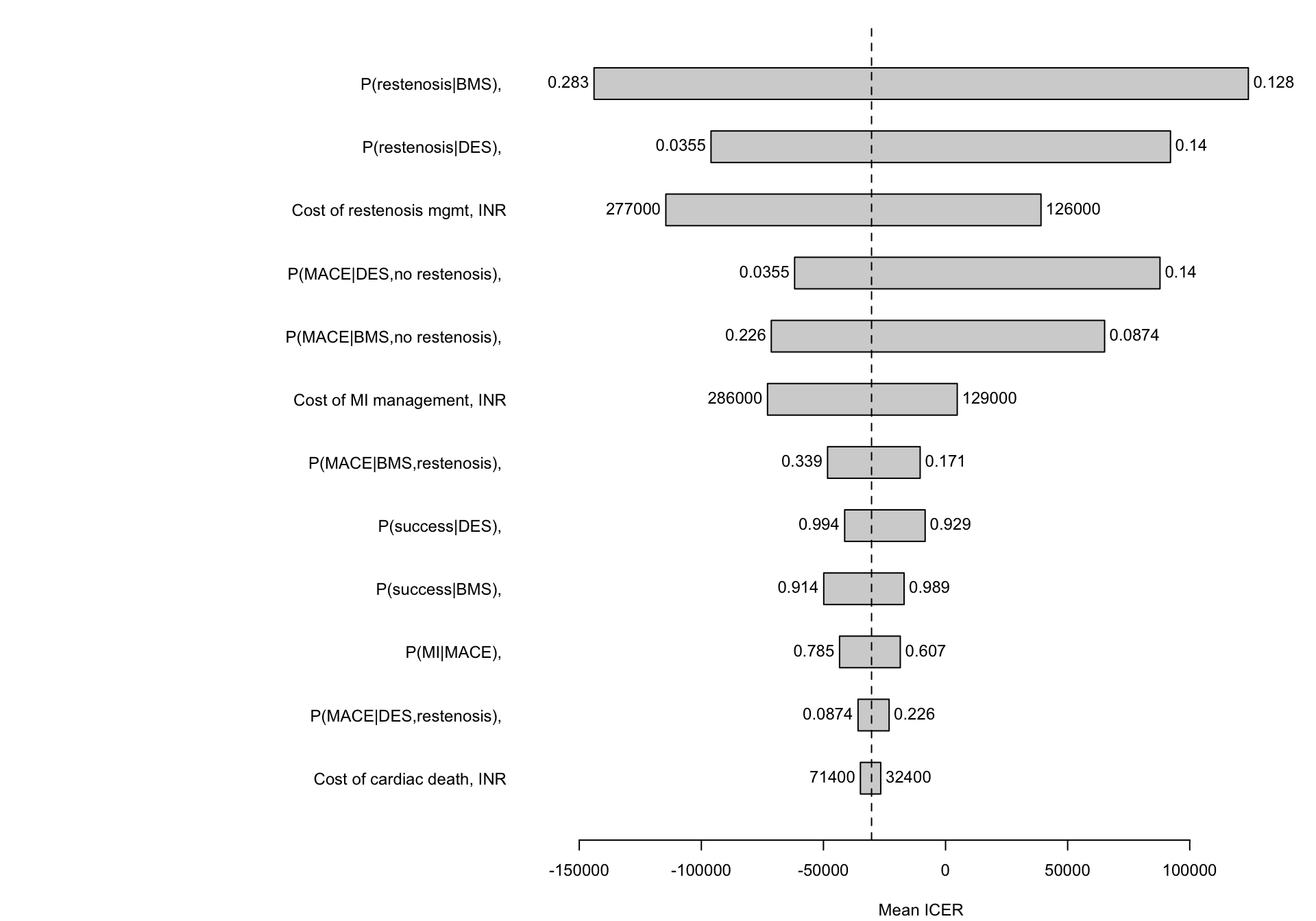
## 10. Built-in Feature: Tornado Diagram (One-way DSA)
The `tornado()` method varies each uncertain parameter over its 95% confidence interval — one at a time — and shows which parameters have the biggest impact on the result. This is **deterministic sensitivity analysis** (DSA), automated.
To use this, we need to rebuild the tree with **model variables** (`ModVar` objects) instead of fixed numbers. This tells `rdecision` the uncertainty distribution for each parameter.
```{r}
#| label: psa-tree-build
#| echo: true
# ============================================================
# REBUILD TREE WITH UNCERTAINTY DISTRIBUTIONS
# ============================================================
# BetaModVar  → probabilities (bounded 0–1)
# GammaModVar → costs (non-negative, right-skewed)

# --- Probability ModVars ---
# Beta distribution: alpha = successes, beta = failures
# Mean = alpha/(alpha+beta)

mv_rest_des <- BetaModVar$new(
  description = "P(restenosis|DES)", units = "", alpha = 8, beta = 92)

mv_rest_bms <- BetaModVar$new(
  description = "P(restenosis|BMS)", units = "", alpha = 20, beta = 80)

mv_mace_des_r <- BetaModVar$new(
  description = "P(MACE|DES,restenosis)", units = "", alpha = 15, beta = 85)

mv_mace_bms_r <- BetaModVar$new(
  description = "P(MACE|BMS,restenosis)", units = "", alpha = 25, beta = 75)

mv_mace_des_nr <- BetaModVar$new(
  description = "P(MACE|DES,no restenosis)", units = "", alpha = 8, beta = 92)

mv_mace_bms_nr <- BetaModVar$new(
  description = "P(MACE|BMS,no restenosis)", units = "", alpha = 15, beta = 85)

mv_p_mi <- BetaModVar$new(
  description = "P(MI|MACE)", units = "", alpha = 70, beta = 30)

mv_p_success_des <- BetaModVar$new(
  description = "P(success|DES)", units = "", alpha = 97, beta = 3)

mv_p_success_bms <- BetaModVar$new(
  description = "P(success|BMS)", units = "", alpha = 96, beta = 4)

# --- Cost ModVars (Gamma distribution) ---
# Gamma: mean = shape × scale; shape = 25 gives ~20% CV
# units = "INR" for Indian Rupees

mv_cost_restenosis <- GammaModVar$new(
  description = "Cost of restenosis mgmt", units = "INR",
  shape = 25, scale = cost_restenosis_mgmt / 25)

mv_cost_mi <- GammaModVar$new(
  description = "Cost of MI management", units = "INR",
  shape = 25, scale = cost_mi_management / 25)

mv_cost_death <- GammaModVar$new(
  description = "Cost of cardiac death", units = "INR",
  shape = 25, scale = cost_cardiac_death_cost / 25)

# ============================================================
# REBUILD NODES (same structure, but with ModVar probabilities)
# ============================================================

# Decision node
d2 <- DecisionNode$new("PCI Stent Choice")

# --- DES arm ---
c2_des_proc    <- ChanceNode$new("DES: Procedure")
c2_des_rest    <- ChanceNode$new("DES: Restenosis?")
c2_des_mace_r  <- ChanceNode$new("DES: MACE (post-restenosis)")
c2_des_mace_nr <- ChanceNode$new("DES: MACE (no restenosis)")
c2_des_mtype_r <- ChanceNode$new("DES: MACE type (rest)")
c2_des_mtype_nr <- ChanceNode$new("DES: MACE type (no rest)")

l2_des_fail      <- LeafNode$new("DES: Fail→CABG",       utility = leaf_u_failure,  interval = leaf_interval)
l2_des_rest_well <- LeafNode$new("DES: Rest→Well",       utility = leaf_u_rest_ok,  interval = leaf_interval)
l2_des_rest_mi   <- LeafNode$new("DES: Rest→MI",         utility = leaf_u_mi,       interval = leaf_interval)
l2_des_rest_death <- LeafNode$new("DES: Rest→Death",     utility = leaf_u_death,    interval = leaf_interval)
l2_des_nr_well   <- LeafNode$new("DES: NoRest→Well",     utility = leaf_u_well,     interval = leaf_interval)
l2_des_nr_mi     <- LeafNode$new("DES: NoRest→MI",       utility = leaf_u_mi,       interval = leaf_interval)
l2_des_nr_death  <- LeafNode$new("DES: NoRest→Death",    utility = leaf_u_death,    interval = leaf_interval)

# --- BMS arm ---
c2_bms_proc    <- ChanceNode$new("BMS: Procedure")
c2_bms_rest    <- ChanceNode$new("BMS: Restenosis?")
c2_bms_mace_r  <- ChanceNode$new("BMS: MACE (post-restenosis)")
c2_bms_mace_nr <- ChanceNode$new("BMS: MACE (no restenosis)")
c2_bms_mtype_r <- ChanceNode$new("BMS: MACE type (rest)")
c2_bms_mtype_nr <- ChanceNode$new("BMS: MACE type (no rest)")

l2_bms_fail      <- LeafNode$new("BMS: Fail→CABG",       utility = leaf_u_failure,  interval = leaf_interval)
l2_bms_rest_well <- LeafNode$new("BMS: Rest→Well",       utility = leaf_u_rest_ok,  interval = leaf_interval)
l2_bms_rest_mi   <- LeafNode$new("BMS: Rest→MI",         utility = leaf_u_mi,       interval = leaf_interval)
l2_bms_rest_death <- LeafNode$new("BMS: Rest→Death",     utility = leaf_u_death,    interval = leaf_interval)
l2_bms_nr_well   <- LeafNode$new("BMS: NoRest→Well",     utility = leaf_u_well,     interval = leaf_interval)
l2_bms_nr_mi     <- LeafNode$new("BMS: NoRest→MI",       utility = leaf_u_mi,       interval = leaf_interval)
l2_bms_nr_death  <- LeafNode$new("BMS: NoRest→Death",    utility = leaf_u_death,    interval = leaf_interval)

# ============================================================
# REBUILD EDGES with ModVar probabilities and costs
# ============================================================

# Decision actions
a2_des <- Action$new(d2, c2_des_proc, cost = 0, label = "DES")
a2_bms <- Action$new(d2, c2_bms_proc, cost = 0, label = "BMS")

# --- DES edges ---
e2_des_succ  <- Reaction$new(c2_des_proc, c2_des_rest,    p = mv_p_success_des, cost = edge_cost_des,         label = "Success")
e2_des_fail  <- Reaction$new(c2_des_proc, l2_des_fail,    p = NA_real_,         cost = edge_cost_failure_des,  label = "Failure")

e2_des_rest  <- Reaction$new(c2_des_rest, c2_des_mace_r,  p = mv_rest_des,      cost = mv_cost_restenosis,    label = "Restenosis")
e2_des_nrest <- Reaction$new(c2_des_rest, c2_des_mace_nr, p = NA_real_,         cost = 0,                     label = "No Restenosis")

e2_des_mace_r_y <- Reaction$new(c2_des_mace_r, c2_des_mtype_r,   p = mv_mace_des_r, cost = 0, label = "MACE")
e2_des_mace_r_n <- Reaction$new(c2_des_mace_r, l2_des_rest_well, p = NA_real_,       cost = 0, label = "No MACE")

e2_des_r_mi    <- Reaction$new(c2_des_mtype_r, l2_des_rest_mi,    p = mv_p_mi,   cost = mv_cost_mi,    label = "MI")
e2_des_r_death <- Reaction$new(c2_des_mtype_r, l2_des_rest_death, p = NA_real_,  cost = mv_cost_death,  label = "Death")

e2_des_mace_nr_y <- Reaction$new(c2_des_mace_nr, c2_des_mtype_nr,  p = mv_mace_des_nr, cost = 0, label = "MACE")
e2_des_mace_nr_n <- Reaction$new(c2_des_mace_nr, l2_des_nr_well,   p = NA_real_,        cost = 0, label = "No MACE")

e2_des_nr_mi    <- Reaction$new(c2_des_mtype_nr, l2_des_nr_mi,    p = mv_p_mi,   cost = mv_cost_mi,    label = "MI")
e2_des_nr_death <- Reaction$new(c2_des_mtype_nr, l2_des_nr_death, p = NA_real_,  cost = mv_cost_death,  label = "Death")

# --- BMS edges ---
e2_bms_succ  <- Reaction$new(c2_bms_proc, c2_bms_rest,    p = mv_p_success_bms, cost = edge_cost_bms,         label = "Success")
e2_bms_fail  <- Reaction$new(c2_bms_proc, l2_bms_fail,    p = NA_real_,         cost = edge_cost_failure_bms,  label = "Failure")

e2_bms_rest  <- Reaction$new(c2_bms_rest, c2_bms_mace_r,  p = mv_rest_bms,      cost = mv_cost_restenosis,    label = "Restenosis")
e2_bms_nrest <- Reaction$new(c2_bms_rest, c2_bms_mace_nr, p = NA_real_,         cost = 0,                     label = "No Restenosis")

e2_bms_mace_r_y <- Reaction$new(c2_bms_mace_r, c2_bms_mtype_r,   p = mv_mace_bms_r, cost = 0, label = "MACE")
e2_bms_mace_r_n <- Reaction$new(c2_bms_mace_r, l2_bms_rest_well, p = NA_real_,       cost = 0, label = "No MACE")

e2_bms_r_mi    <- Reaction$new(c2_bms_mtype_r, l2_bms_rest_mi,    p = mv_p_mi,   cost = mv_cost_mi,    label = "MI")
e2_bms_r_death <- Reaction$new(c2_bms_mtype_r, l2_bms_rest_death, p = NA_real_,  cost = mv_cost_death,  label = "Death")

e2_bms_mace_nr_y <- Reaction$new(c2_bms_mace_nr, c2_bms_mtype_nr,  p = mv_mace_bms_nr, cost = 0, label = "MACE")
e2_bms_mace_nr_n <- Reaction$new(c2_bms_mace_nr, l2_bms_nr_well,   p = NA_real_,        cost = 0, label = "No MACE")

e2_bms_nr_mi    <- Reaction$new(c2_bms_mtype_nr, l2_bms_nr_mi,    p = mv_p_mi,   cost = mv_cost_mi,    label = "MI")
e2_bms_nr_death <- Reaction$new(c2_bms_mtype_nr, l2_bms_nr_death, p = NA_real_,  cost = mv_cost_death,  label = "Death")

# ============================================================
# ASSEMBLE the PSA-ready tree
# ============================================================

V2 <- list(
  d2,
  c2_des_proc, c2_des_rest, c2_des_mace_r, c2_des_mace_nr, c2_des_mtype_r, c2_des_mtype_nr,
  l2_des_fail, l2_des_rest_well, l2_des_rest_mi, l2_des_rest_death,
  l2_des_nr_well, l2_des_nr_mi, l2_des_nr_death,
  c2_bms_proc, c2_bms_rest, c2_bms_mace_r, c2_bms_mace_nr, c2_bms_mtype_r, c2_bms_mtype_nr,
  l2_bms_fail, l2_bms_rest_well, l2_bms_rest_mi, l2_bms_rest_death,
  l2_bms_nr_well, l2_bms_nr_mi, l2_bms_nr_death
)

E2 <- list(
  a2_des, a2_bms,
  e2_des_succ, e2_des_fail, e2_des_rest, e2_des_nrest,
  e2_des_mace_r_y, e2_des_mace_r_n, e2_des_r_mi, e2_des_r_death,
  e2_des_mace_nr_y, e2_des_mace_nr_n, e2_des_nr_mi, e2_des_nr_death,
  e2_bms_succ, e2_bms_fail, e2_bms_rest, e2_bms_nrest,
  e2_bms_mace_r_y, e2_bms_mace_r_n, e2_bms_r_mi, e2_bms_r_death,
  e2_bms_mace_nr_y, e2_bms_mace_nr_n, e2_bms_nr_mi, e2_bms_nr_death
)

dt_psa <- DecisionTree$new(V2, E2)
```
::: {.callout-important}
## Same tree, now with uncertainty
The tree structure is identical to Section 5–6. The only difference is that probabilities and costs are now `ModVar` objects (Beta and Gamma distributions) instead of fixed numbers. This is all `rdecision` needs to run both DSA and PSA.
:::
Now the tornado diagram — **one line**:
```{r}
#| label: fig-tornado
#| echo: true
#| fig-cap: "Tornado diagram: which parameters matter most for the ICER?"
#| fig-width: 10
#| fig-height: 7
# Tornado: vary each parameter over its 95% CI
# index = DES strategy, ref = BMS strategy
to <- dt_psa$tornado(
  index = a2_des,
  ref   = a2_bms,
  outcome = "ICER",
  draw = TRUE
)
```
::: {.callout-note}
## Reading the tornado
Each bar shows how the **ICER** (DES vs BMS) changes when that one parameter is varied from its lower to upper 95% confidence limit, with all other parameters held at their mean. The longest bars are the parameters that matter most — these are where you should focus your evidence gathering.
:::
```{r}
#| label: tornado-table
#| echo: true
# The tornado also returns a data frame with the numeric values
kable(to, digits = 0,
      caption = "Tornado diagram values: ICER sensitivity to each parameter")
```
## 11. Built-in Feature: Probabilistic Sensitivity Analysis (PSA)
This is where `rdecision` truly earns its keep. Instead of writing sampling loops, we call `evaluate()` with `setvars = "random"` and get 1,000 Monte Carlo iterations — automatically.
```{r}
#| label: run-psa
#| echo: true
# ============================================================
# RUN PSA — 1,000 iterations, one line!
# ============================================================
set.seed(42)  # for reproducibility
N_psa <- 1000L

psa_results <- dt_psa$evaluate(setvars = "random", by = "run", N = N_psa)

cat("PSA returned:", nrow(psa_results), "rows x", ncol(psa_results), "columns\n")
cat("Column names:", paste(names(psa_results), collapse = ", "), "\n")
kable(head(psa_results, 5), digits = 2,
      caption = "First 5 PSA iterations (of 1,000)")
```
::: {.callout-warning}
## Compare with the manual approach
To do the same thing manually, you would write a `for`-loop that samples from `rbeta()` and `rgamma()`, calls `run_model()` 1,000 times, and binds the results into a data frame — about 25–30 lines of code. Here it's **one line**: `dt_psa$evaluate(setvars = "random", by = "run", N = 1000)`.
:::
## 12. Visualising PSA Results: CE Plane and CEAC
With 1,000 iterations in hand, we can build the two most important PSA visualisations.
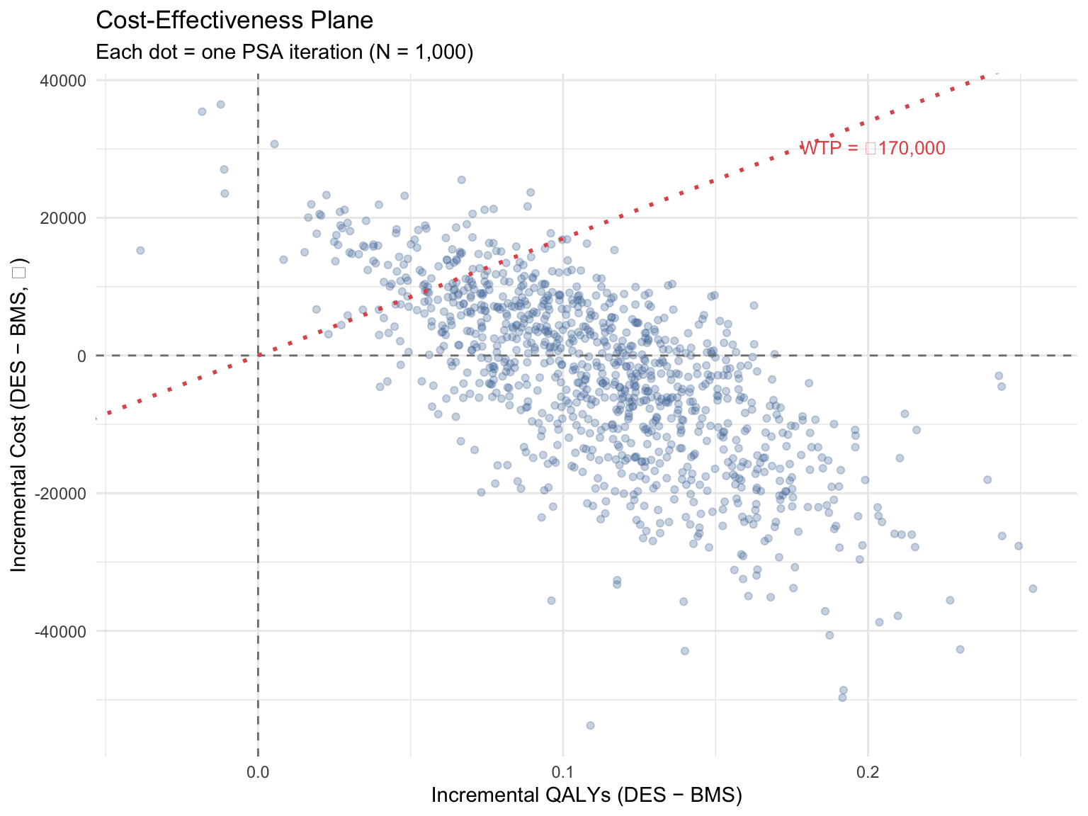
### 12a. Cost-Effectiveness Plane
```{r}
#| label: fig-ce-plane
#| echo: true
#| fig-cap: "Cost-effectiveness plane: 1,000 PSA iterations (DES vs BMS)"
#| fig-width: 8
#| fig-height: 6
library(ggplot2)
# PSA with by="run" returns WIDE format: one row per iteration
# Columns: Run, Cost.DES, Cost.BMS, QALY.DES, QALY.BMS, etc.
inc_cost <- psa_results$Cost.DES - psa_results$Cost.BMS
inc_qaly <- psa_results$QALY.DES - psa_results$QALY.BMS

ce_data <- data.frame(
  inc_cost = inc_cost,
  inc_qaly = inc_qaly
)

# WTP threshold line (1× GDP per capita India)
wtp <- 170000

ggplot(ce_data, aes(x = inc_qaly, y = inc_cost)) +
  geom_point(alpha = 0.3, colour = "#4e79a7", size = 1.5) +
  geom_hline(yintercept = 0, linetype = "dashed", colour = "grey50") +
  geom_vline(xintercept = 0, linetype = "dashed", colour = "grey50") +
  geom_abline(intercept = 0, slope = wtp, linetype = "dotted",
              colour = "#e15759", linewidth = 1) +
  annotate("text", x = max(inc_qaly) * 0.7, y = wtp * max(inc_qaly) * 0.7,
           label = paste0("WTP = ₹", format(wtp, big.mark = ",")),
           colour = "#e15759", hjust = 0, size = 3.5) +
  labs(x = "Incremental QALYs (DES − BMS)",
       y = "Incremental Cost (DES − BMS, ₹)",
       title = "Cost-Effectiveness Plane",
       subtitle = "Each dot = one PSA iteration (N = 1,000)") +
  theme_minimal()
```
::: {.callout-tip}
## Reading the CE plane
**Southeast quadrant** (right, below zero) = DES is dominant (better and cheaper). **Northeast below the WTP line** = DES is cost-effective. Points **above the WTP line** = DES is not cost-effective at that threshold. The cloud of points shows the uncertainty in the conclusion.
:::
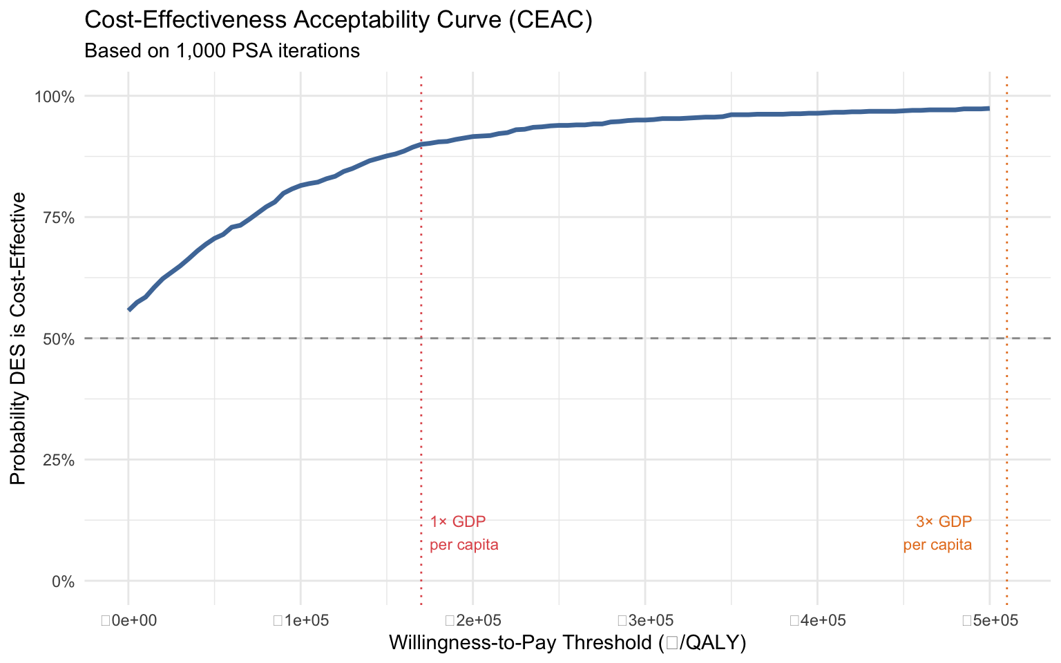
### 12b. Cost-Effectiveness Acceptability Curve (CEAC)
The CEAC answers: **"At any given WTP threshold, what is the probability that DES is cost-effective?"**
```{r}
#| label: fig-ceac
#| echo: true
#| fig-cap: "Cost-Effectiveness Acceptability Curve: probability of DES being cost-effective"
#| fig-width: 8
#| fig-height: 5
# Generate CEAC: sweep WTP from 0 to ₹5,00,000
wtp_range <- seq(0, 500000, by = 5000)

# For each WTP, compute proportion of iterations where DES is cost-effective
# DES is CE if: inc_cost / inc_qaly < WTP, or equivalently: inc_cost - WTP * inc_qaly < 0
prob_ce <- sapply(wtp_range, function(w) {
  nmb <- inc_qaly * w - inc_cost  # net monetary benefit
  mean(nmb > 0)
})

ceac_data <- data.frame(WTP = wtp_range, Prob_CE = prob_ce)

ggplot(ceac_data, aes(x = WTP, y = Prob_CE)) +
  geom_line(colour = "#4e79a7", linewidth = 1.2) +
  geom_hline(yintercept = 0.5, linetype = "dashed", colour = "grey60") +
  geom_vline(xintercept = 170000, linetype = "dotted", colour = "#e15759") +
  annotate("text", x = 175000, y = 0.1,
           label = "1× GDP\nper capita",
           colour = "#e15759", hjust = 0, size = 3) +
  geom_vline(xintercept = 510000, linetype = "dotted", colour = "#e67e22") +
  annotate("text", x = 490000, y = 0.1,
           label = "3× GDP\nper capita",
           colour = "#e67e22", hjust = 1, size = 3) +
  scale_x_continuous(labels = function(x) paste0("₹", format(x, big.mark = ","))) +
  scale_y_continuous(labels = scales::percent_format(), limits = c(0, 1)) +
  labs(x = "Willingness-to-Pay Threshold (₹/QALY)",
       y = "Probability DES is Cost-Effective",
       title = "Cost-Effectiveness Acceptability Curve (CEAC)",
       subtitle = "Based on 1,000 PSA iterations") +
  theme_minimal()
```
::: {.callout-important}
## The policy answer
A single ICER says "DES is cost-effective." The CEAC says "DES is cost-effective with **X% probability** at threshold Y." This is what decision-makers actually need. Notice how we generated this entire analysis — PSA, CE plane, CEAC — with `rdecision` doing the heavy lifting.
:::
## 13. Summary: Package Features at a Glance
```{r}
#| label: feature-summary
#| echo: false
features <- data.frame(
Feature = c(
"Tree structure as code",
"Automatic rollback (evaluate)",
"Tree diagram (draw)",
"DOT/GraphViz export",
"Tornado diagram (DSA)",
"PSA with ModVar distributions",
"CE plane scatter plot",
"CEAC curve",
"Semi-Markov models"
),
Status = c(
"Demonstrated above (Sections 5–7)",
"Demonstrated above (Section 7)",
"Demonstrated above (Section 9)",
"Demonstrated above (Section 9)",
"Demonstrated above (Section 10)",
"Demonstrated above (Section 11)",
"Demonstrated above (Section 12a)",
"Demonstrated above (Section 12b)",
"Available — not shown (Day 2 topic)"
),
Manual_Equivalent = c(
"~50 lines of R arithmetic",
"~80 lines (Sections 6–9 in Session 4)",
"Separate DiagrammeR code",
"Not available without extra packages",
"Write your own loop + plotting code",
"~25–30 lines (for-loop + rbeta/rgamma)",
"Manual ggplot from loop results",
"Manual ggplot from loop results",
"Requires custom state-transition code"
)
)
kable(features,
col.names = c("Feature", "Where Shown", "Manual Equivalent"),
caption = "rdecision built-in features demonstrated in this document",
align = c("l", "l", "l"))
```
## 14. When to Use Which Approach
```{r}
#| label: when-to-use
#| echo: false
guidance <- data.frame(
Scenario = c("Learning HTA / teaching students",
"Small decision tree (< 10 pathways)",
"Complex tree with many branches",
"Production HTA submission",
"Need PSA / VOI analysis",
"Need full audit trail",
"Quick one-off analysis"),
Recommended = c("Manual first, then rdecision",
"Either — manual is fine",
"rdecision package",
"rdecision (or heemod for Markov)",
"rdecision — built-in support",
"rdecision — formal model structure",
"Manual — faster to set up")
)
kable(guidance,
col.names = c("Scenario", "Recommended Approach"),
caption = "Choosing between manual and package-based modelling",
align = c("l", "l"))
```
::: {.callout-tip}
## The learning progression
1. **Session 4**: Build from scratch → understand every calculation
2. **This tab**: Same model in `rdecision` → see how packages structure it, then use built-in DSA, PSA, CEAC
3. **DSA/PSA sessions**: Deep dive into sensitivity analysis theory
4. **Your own HTA**: Choose the right tool for the job
:::
## Key Takeaways
The manual approach and the `rdecision` package are **complementary**, not competing. The manual model teaches you *what* is being calculated; the package handles *how* to do it efficiently at scale.
What we demonstrated in this document:
1. **Same model, same results** — manual and `rdecision` cross-validate
2. **Tree drawing** — `dt$draw()` produces a diagram directly from the model
3. **Tornado diagram** — `dt$tornado()` does one-way DSA in one line
4. **PSA** — `dt$evaluate(setvars = "random", N = 1000)` runs 1,000 Monte Carlo iterations
5. **CE plane and CEAC** — built from PSA results with standard `ggplot2`
The entire analysis — from model definition to policy-relevant uncertainty quantification — is reproducible and contained in a single `.qmd` file.
## References
- Sims A (2024). rdecision: Decision Analytic Modelling in Health Economics. R package. [CRAN](https://cran.r-project.org/package=rdecision)
- Jenks M et al. (2016). Clinical and economic burden of surgical site infection. *Journal of Hospital Infection*.
- Briggs A, Sculpher M, Claxton K (2006). *Decision Modelling for Health Economic Evaluation*. Oxford University Press.
- R-HTA Consortium. [R for Health Technology Assessment](https://r-hta.org/)
> **Back to Session 4:** The manual step-by-step model is in `des-bms-decision-tree.qmd`. Use it as your reference for understanding; use this tab for seeing how packages streamline the process.