---
title: "Session 9: PSA for the Partitioned Survival Model"
subtitle: "Quantifying uncertainty in the trastuzumab cost-effectiveness analysis"
format:
html:
toc: true
code-fold: show
---
## Introduction
Probabilistic Sensitivity Analysis (PSA) quantifies how parameter uncertainty affects model outputs. We introduced PSA in Session 6 for Markov models—the same principle applies to Partitioned Survival Models (PSMs). The workflow is identical: sample parameters from their distributions, run the model for each sample, and collect results to build distributions of costs, effects, and cost-effectiveness.
This session applies PSA to the breast cancer trastuzumab model from Session 8, allowing us to quantify uncertainty in the incremental cost-effectiveness ratio (ICER) and present decision uncertainty to stakeholders.
## Setting up R environment
```{r}
#| message: false
library(tidyverse)
library(ggplot2)
library(gridExtra)

# Set theme for plots
theme_set(theme_minimal() +
          theme(panel.grid.major = element_line(colour = "grey90"),
                panel.grid.minor = element_blank()))
```
## Define parameter distributions
We specify probability distributions for key model parameters. The choice of distribution reflects our beliefs about parameter uncertainty.
```{r}
# Define parameter distributions

## Hazard ratios (log-normal distribution)
hr_os_mean <- log(0.70)        # Log mean for OS HR
hr_os_sd <- 0.15               # Log SD
hr_pfs_mean <- log(0.50)       # Log mean for PFS HR
hr_pfs_sd <- 0.20              # Log SD

## Costs (gamma distribution) in INR
cost_pf_trast_yr1_mean <- 420000   # Year 1 trastuzumab cost
cost_pf_trast_yr1_sd <- 80000      # SD ~19% of mean
cost_pd_mean <- 180000             # Progressive disease cost
cost_pd_sd <- 40000                # SD ~22% of mean

## Utilities (beta distribution)
utility_pf_mean <- 0.80
utility_pf_sd <- 0.05
utility_pd_mean <- 0.55
utility_pd_sd <- 0.08

# Base case Weibull parameters (control arm)
os_lambda_ctrl <- 0.045
os_gamma_ctrl <- 1.15
pfs_lambda_ctrl <- 0.12
pfs_gamma_ctrl <- 1.05

# Year 1 maintenance cost for trastuzumab
cost_trast_maintenance_yr1 <- 25000
```
## Helper functions: Convert mean/SD to distribution parameters
For gamma distributions: shape and rate parameters are derived from desired mean and SD.
For beta distributions: alpha and beta parameters are derived from desired mean and SD.
```{r}
# Convert mean and SD to gamma shape and rate parameters
mean_sd_to_gamma <- function(mean, sd) {
  rate <- mean / (sd^2)
  shape <- mean * rate
  return(list(shape = shape, rate = rate))
}

# Convert mean and SD to beta shape parameters
mean_sd_to_beta <- function(mean, sd) {
  # Using method of moments
  # Constraint: mean must be between 0 and 1 for beta
  if (mean <= 0 | mean >= 1) {
    stop("Beta mean must be strictly between 0 and 1")
  }

  alpha <- ((1 - mean) / (sd^2) - 1 / mean) * mean^2
  beta <- alpha * (1 / mean - 1)

  return(list(alpha = alpha, beta = beta))
}

# Test the functions
cat("Gamma conversion (cost_pd): mean=180000, sd=40000\n")
gamma_params_cost_pd <- mean_sd_to_gamma(cost_pd_mean, cost_pd_sd)
print(gamma_params_cost_pd)
cat("\nBeta conversion (utility_pf): mean=0.80, sd=0.05\n")
beta_params_utility_pf <- mean_sd_to_beta(utility_pf_mean, utility_pf_sd)
print(beta_params_utility_pf)
```
## Partitioned Survival Model function
The PSM function from Session 8, adapted to accept sampled parameters:
```{r}
psm_model <- function(
    hr_os = 0.70,
    hr_pfs = 0.50,
    os_lambda_ctrl = 0.045,
    os_gamma_ctrl = 1.15,
    pfs_lambda_ctrl = 0.12,
    pfs_gamma_ctrl = 1.05,
    cost_pf_trast = 420000,
    cost_pd = 180000,
    utility_pf = 0.80,
    utility_pd = 0.55,
    cost_trast_maint = 25000,
    time_horizon = 20,
    discount_rate = 0.03
) {

  # Time steps (annual)
  times <- seq(0, time_horizon, by = 1)

  ## Control arm: survival functions
  S_os_ctrl <- function(t) exp(-os_lambda_ctrl * t^os_gamma_ctrl)
  S_pfs_ctrl <- function(t) exp(-pfs_lambda_ctrl * t^pfs_gamma_ctrl)

  # Trastuzumab arm: scale lambda by HR (proportional hazards, matching Session 8)
  S_os_trast <- function(t) exp(-(os_lambda_ctrl * hr_os) * t^os_gamma_ctrl)
  S_pfs_trast <- function(t) exp(-(pfs_lambda_ctrl * hr_pfs) * t^pfs_gamma_ctrl)

  ## State occupancy (trapezoid rule approximation)
  df <- tibble(
    time = times,
    S_os_ctrl_t = sapply(times, S_os_ctrl),
    S_pfs_ctrl_t = sapply(times, S_pfs_ctrl),
    S_os_trast_t = sapply(times, S_os_trast),
    S_pfs_trast_t = sapply(times, S_pfs_trast)
  ) %>%
    mutate(
      # PFS occupancy
      pfs_ctrl_t = S_pfs_ctrl_t,
      pfs_trast_t = S_pfs_trast_t,
      # PD occupancy (OS - PFS)
      pd_ctrl_t = pmax(S_os_ctrl_t - S_pfs_ctrl_t, 0),
      pd_trast_t = pmax(S_os_trast_t - S_pfs_trast_t, 0),
      # Dead occupancy
      dead_ctrl_t = 1 - S_os_ctrl_t,
      dead_trast_t = 1 - S_os_trast_t
    )

  ## Cycle values (apply half-cycle correction)
  df <- df %>%
    mutate(
      # Discount factors (applied at mid-cycle for annual cycles)
      discount = (1 + discount_rate)^(-(time - 0.5))
    )

  ## Costs
  # Trastuzumab: Year 1 cost in PFS states, maintenance thereafter
  df <- df %>%
    mutate(
      cost_trast_pfs = if_else(
        time <= 1,
        cost_pf_trast,
        cost_trast_maint
      ),
      cost_pf_ctrl = 0,
      cost_pf_trast = cost_trast_pfs,
      cost_pd_ctrl = cost_pd,
      cost_pd_trast = cost_pd,
      cost_dead = 0
    )

  # Expected costs per arm (cycle costs × occupancy)
  df <- df %>%
    mutate(
      total_cost_ctrl = pfs_ctrl_t * cost_pf_ctrl + pd_ctrl_t * cost_pd_ctrl + dead_ctrl_t * cost_dead,
      total_cost_trast = pfs_trast_t * cost_pf_trast + pd_trast_t * cost_pd_trast + dead_trast_t * cost_dead
    )

  ## QALYs
  df <- df %>%
    mutate(
      utility_pf = utility_pf,
      utility_pd = utility_pd,
      utility_dead = 0,
      total_qaly_ctrl = pfs_ctrl_t * utility_pf + pd_ctrl_t * utility_pd + dead_ctrl_t * utility_dead,
      total_qaly_trast = pfs_trast_t * utility_pf + pd_trast_t * utility_pd + dead_trast_t * utility_dead
    )

  ## Discounted totals (per cycle per person)
  df <- df %>%
    mutate(
      disc_cost_ctrl = total_cost_ctrl * discount,
      disc_cost_trast = total_cost_trast * discount,
      disc_qaly_ctrl = total_qaly_ctrl * discount,
      disc_qaly_trast = total_qaly_trast * discount
    )

  ## Summary results (undiscounted and discounted)
  results <- list(
    cost_ctrl = sum(df$disc_cost_ctrl),
    cost_trast = sum(df$disc_cost_trast),
    qaly_ctrl = sum(df$disc_qaly_ctrl),
    qaly_trast = sum(df$disc_qaly_trast),
    inc_cost = sum(df$disc_cost_trast) - sum(df$disc_cost_ctrl),
    inc_qaly = sum(df$disc_qaly_trast) - sum(df$disc_qaly_ctrl),
    icer = ifelse(
      abs(sum(df$disc_qaly_trast) - sum(df$disc_qaly_ctrl)) < 1e-9,
      NA_real_,
      (sum(df$disc_cost_trast) - sum(df$disc_cost_ctrl)) /
        (sum(df$disc_qaly_trast) - sum(df$disc_qaly_ctrl))
    )
  )

  return(results)
}

# Test with base case
base_case <- psm_model()
cat("\n=== Base case results ===\n")
cat("ICER: ₹", format(round(base_case$icer, 0), big.mark = ","), "/QALY\n", sep = "")
cat("Inc. Cost: ₹", format(round(base_case$inc_cost, 0), big.mark = ","), "\n", sep = "")
cat("Inc. QALY: ", round(base_case$inc_qaly, 3), "\n", sep = "")
```
## Run Probabilistic Sensitivity Analysis
We conduct 3,000 PSA iterations, sampling parameters from their distributions for each iteration.
```{r}
#| cache: true
set.seed(2026)
n_iterations <- 3000

# Pre-allocate storage
psa_results <- tibble(
  iteration = integer(n_iterations),
  hr_os = numeric(n_iterations),
  hr_pfs = numeric(n_iterations),
  cost_pf_trast_yr1 = numeric(n_iterations),
  cost_pd = numeric(n_iterations),
  utility_pf = numeric(n_iterations),
  utility_pd = numeric(n_iterations),
  cost_ctrl = numeric(n_iterations),
  cost_trast = numeric(n_iterations),
  qaly_ctrl = numeric(n_iterations),
  qaly_trast = numeric(n_iterations),
  inc_cost = numeric(n_iterations),
  inc_qaly = numeric(n_iterations),
  icer = numeric(n_iterations)
)

# Run PSA
for (i in seq_len(n_iterations)) {

  # Sample parameters
  hr_os_sampled <- exp(rnorm(1, hr_os_mean, hr_os_sd))
  hr_pfs_sampled <- exp(rnorm(1, hr_pfs_mean, hr_pfs_sd))

  # Gamma distributions for costs
  gamma_pf_trast <- mean_sd_to_gamma(cost_pf_trast_yr1_mean, cost_pf_trast_yr1_sd)
  cost_pf_trast_sampled <- rgamma(1, shape = gamma_pf_trast$shape, rate = gamma_pf_trast$rate)

  gamma_pd <- mean_sd_to_gamma(cost_pd_mean, cost_pd_sd)
  cost_pd_sampled <- rgamma(1, shape = gamma_pd$shape, rate = gamma_pd$rate)

  # Beta distributions for utilities
  beta_pf <- mean_sd_to_beta(utility_pf_mean, utility_pf_sd)
  utility_pf_sampled <- rbeta(1, shape1 = beta_pf$alpha, shape2 = beta_pf$beta)

  beta_pd <- mean_sd_to_beta(utility_pd_mean, utility_pd_sd)
  utility_pd_sampled <- rbeta(1, shape1 = beta_pd$alpha, shape2 = beta_pd$beta)

  # Run model with sampled parameters
  model_output <- psm_model(
    hr_os = hr_os_sampled,
    hr_pfs = hr_pfs_sampled,
    cost_pf_trast = cost_pf_trast_sampled,
    cost_pd = cost_pd_sampled,
    utility_pf = utility_pf_sampled,
    utility_pd = utility_pd_sampled,
    cost_trast_maint = cost_trast_maintenance_yr1
  )

  # Store results
  psa_results$iteration[i] <- i
  psa_results$hr_os[i] <- hr_os_sampled
  psa_results$hr_pfs[i] <- hr_pfs_sampled
  psa_results$cost_pf_trast_yr1[i] <- cost_pf_trast_sampled
  psa_results$cost_pd[i] <- cost_pd_sampled
  psa_results$utility_pf[i] <- utility_pf_sampled
  psa_results$utility_pd[i] <- utility_pd_sampled
  psa_results$cost_ctrl[i] <- model_output$cost_ctrl
  psa_results$cost_trast[i] <- model_output$cost_trast
  psa_results$qaly_ctrl[i] <- model_output$qaly_ctrl
  psa_results$qaly_trast[i] <- model_output$qaly_trast
  psa_results$inc_cost[i] <- model_output$inc_cost
  psa_results$inc_qaly[i] <- model_output$inc_qaly
  psa_results$icer[i] <- model_output$icer

  # Progress message
  if (i %% 500 == 0) {
    cat("Completed iteration", i, "of", n_iterations, "\n")
  }
}
cat("PSA complete!\n")
```
## PSA Results Summary
```{r}
#| label: psa-summary
#| echo: true
library(knitr)

wtp_threshold <- 170000

# Compute NMB for each iteration (unambiguous, unlike ICER)
psa_results <- psa_results %>%
  mutate(
    inc_nmb = wtp_threshold * inc_qaly - inc_cost
  )

# Summary table
psa_summary <- data.frame(
  Metric = c(
    "Mean Incremental Cost",
    "  95% CrI",
    "Mean Incremental QALYs",
    "  95% CrI",
    "Mean ICER",
    "Median ICER",
    "Mean Incremental NMB",
    "  95% CrI",
    paste0("P(cost-effective) at WTP = ₹", format(wtp_threshold, big.mark = ",")),
    "P(dominant)"
  ),
  Value = c(
    paste0("₹", format(round(mean(psa_results$inc_cost)), big.mark = ",")),
    paste0("[₹", format(round(quantile(psa_results$inc_cost, 0.025)), big.mark = ","),
           " to ₹", format(round(quantile(psa_results$inc_cost, 0.975)), big.mark = ","), "]"),
    round(mean(psa_results$inc_qaly), 3),
    paste0("[", round(quantile(psa_results$inc_qaly, 0.025), 3),
           " to ", round(quantile(psa_results$inc_qaly, 0.975), 3), "]"),
    paste0("₹", format(round(mean(psa_results$icer, na.rm = TRUE)), big.mark = ",")),
    paste0("₹", format(round(median(psa_results$icer, na.rm = TRUE)), big.mark = ",")),
    paste0("₹", format(round(mean(psa_results$inc_nmb)), big.mark = ",")),
    paste0("[₹", format(round(quantile(psa_results$inc_nmb, 0.025)), big.mark = ","),
           " to ₹", format(round(quantile(psa_results$inc_nmb, 0.975)), big.mark = ","), "]"),
    paste0(round(mean(psa_results$inc_nmb > 0) * 100, 1), "%"),
    paste0(round(mean(psa_results$inc_cost < 0 & psa_results$inc_qaly > 0) * 100, 1), "%")
  ),
  check.names = FALSE
)

kable(psa_summary, caption = paste0("PSA summary (", n_iterations, " iterations)"))
```
::: {.callout-tip}
## Why NMB in PSA?
Recall from Session 5: you can't meaningfully average ICERs across PSA iterations — a few extreme values (near-zero denominators) can distort the mean. The **incremental NMB** (ΔNMB = WTP × ΔQALYs − ΔCost) has no such problem. A positive mean ΔNMB means the intervention is cost-effective on average. The CEAC below is also based on NMB: at each WTP, it counts what fraction of iterations have ΔNMB > 0.
:::
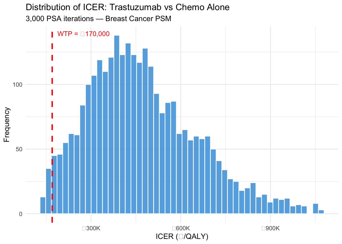
## ICER Distribution
```{r}
#| label: fig-icer-histogram
#| echo: true
#| fig-cap: "Distribution of ICER estimates from 3,000 PSA iterations"
# Filter extreme values for better viz
icer_valid <- psa_results$icer[!is.na(psa_results$icer)]
icer_plot <- icer_valid[icer_valid > quantile(icer_valid, 0.02) &
                         icer_valid < quantile(icer_valid, 0.98)]

ggplot(data.frame(ICER = icer_plot), aes(x = ICER)) +
  geom_histogram(bins = 50, fill = "#3498db", colour = "white", alpha = 0.8) +
  geom_vline(xintercept = 170000, colour = "red", linetype = "dashed", linewidth = 1) +
  annotate("text", x = 170000, y = Inf, label = "WTP = ₹170,000",
           colour = "red", hjust = -0.1, vjust = 2, size = 3.5) +
  scale_x_continuous(labels = function(x) paste0("₹", format(round(x/1000), big.mark=","), "K")) +
  labs(x = "ICER (₹/QALY)", y = "Frequency",
       title = "Distribution of ICER: Trastuzumab vs Chemo Alone",
       subtitle = "3,000 PSA iterations — Breast Cancer PSM") +
  theme_minimal()
```
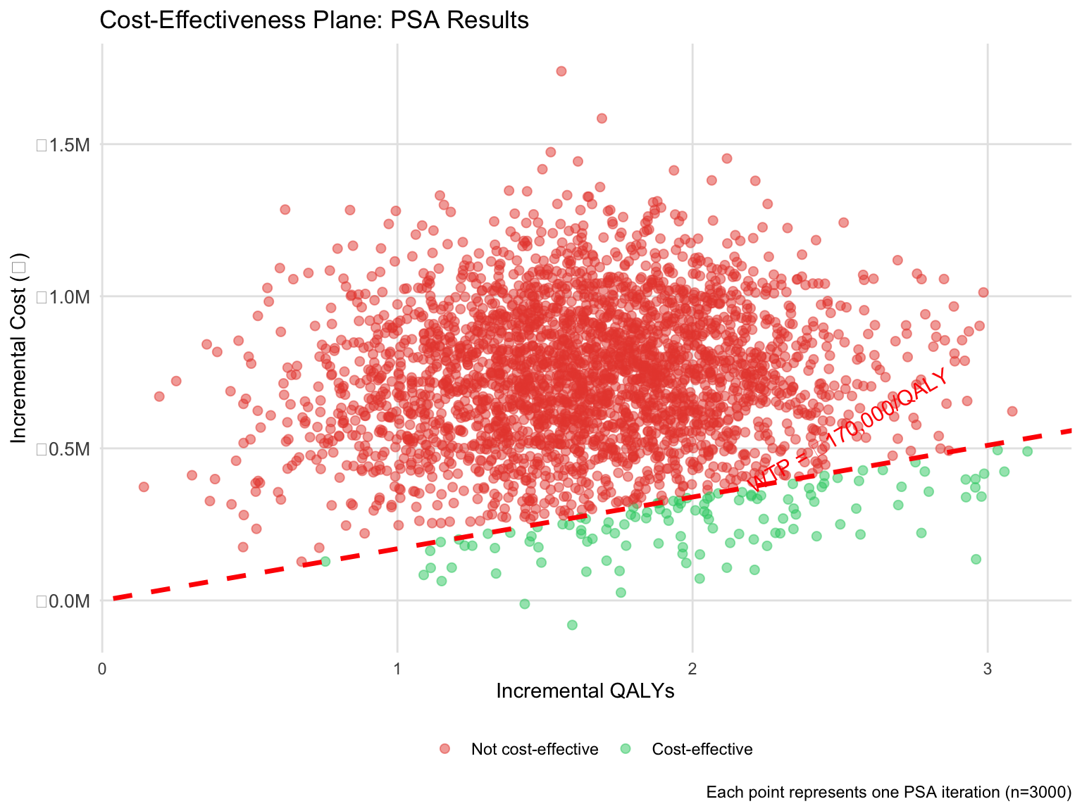
## Cost-Effectiveness Plane
The CE plane shows the relationship between incremental cost and incremental effect for each PSA iteration. The willingness-to-pay (WTP) line at ₹170,000/QALY represents a threshold (approximately 1× GDP per capita for India).
```{r}
#| fig-width: 8
#| fig-height: 6
wtp_threshold <- 170000

# Add CE classification
psa_results <- psa_results %>%
  mutate(
    ce_at_threshold = inc_cost <= (wtp_threshold * inc_qaly),
    quadrant = case_when(
      inc_qaly >= 0 & inc_cost >= 0 ~ "NE (More expensive, more effective)",
      inc_qaly >= 0 & inc_cost < 0 ~ "SE (Cheaper, more effective)",
      inc_qaly < 0 & inc_cost >= 0 ~ "NW (More expensive, less effective)",
      inc_qaly < 0 & inc_cost < 0 ~ "SW (Cheaper, less effective)"
    )
  )

# CE plane plot
p_ce <- ggplot(psa_results, aes(x = inc_qaly, y = inc_cost, colour = ce_at_threshold)) +
  geom_point(alpha = 0.5, size = 2) +
  geom_abline(intercept = 0, slope = wtp_threshold,
              linetype = "dashed", colour = "red", linewidth = 1.2) +
  annotate("text", x = max(psa_results$inc_qaly) * 0.7,
           y = wtp_threshold * max(psa_results$inc_qaly) * 0.7,
           label = "WTP = ₹170,000/QALY", angle = 30,
           colour = "red", size = 4, hjust = 0) +
  scale_colour_manual(
    values = c("TRUE" = "#2ecc71", "FALSE" = "#e74c3c"),
    labels = c("TRUE" = "Cost-effective", "FALSE" = "Not cost-effective"),
    name = ""
  ) +
  labs(
    title = "Cost-Effectiveness Plane: PSA Results",
    x = "Incremental QALYs",
    y = "Incremental Cost (₹)",
    caption = "Each point represents one PSA iteration (n=3000)"
  ) +
  theme(
    legend.position = "bottom",
    axis.text.y = element_text(size = 10)
  ) +
  scale_y_continuous(labels = function(x) paste0("₹", format(round(x/1e6, 1), nsmall = 1), "M"))

print(p_ce)
```
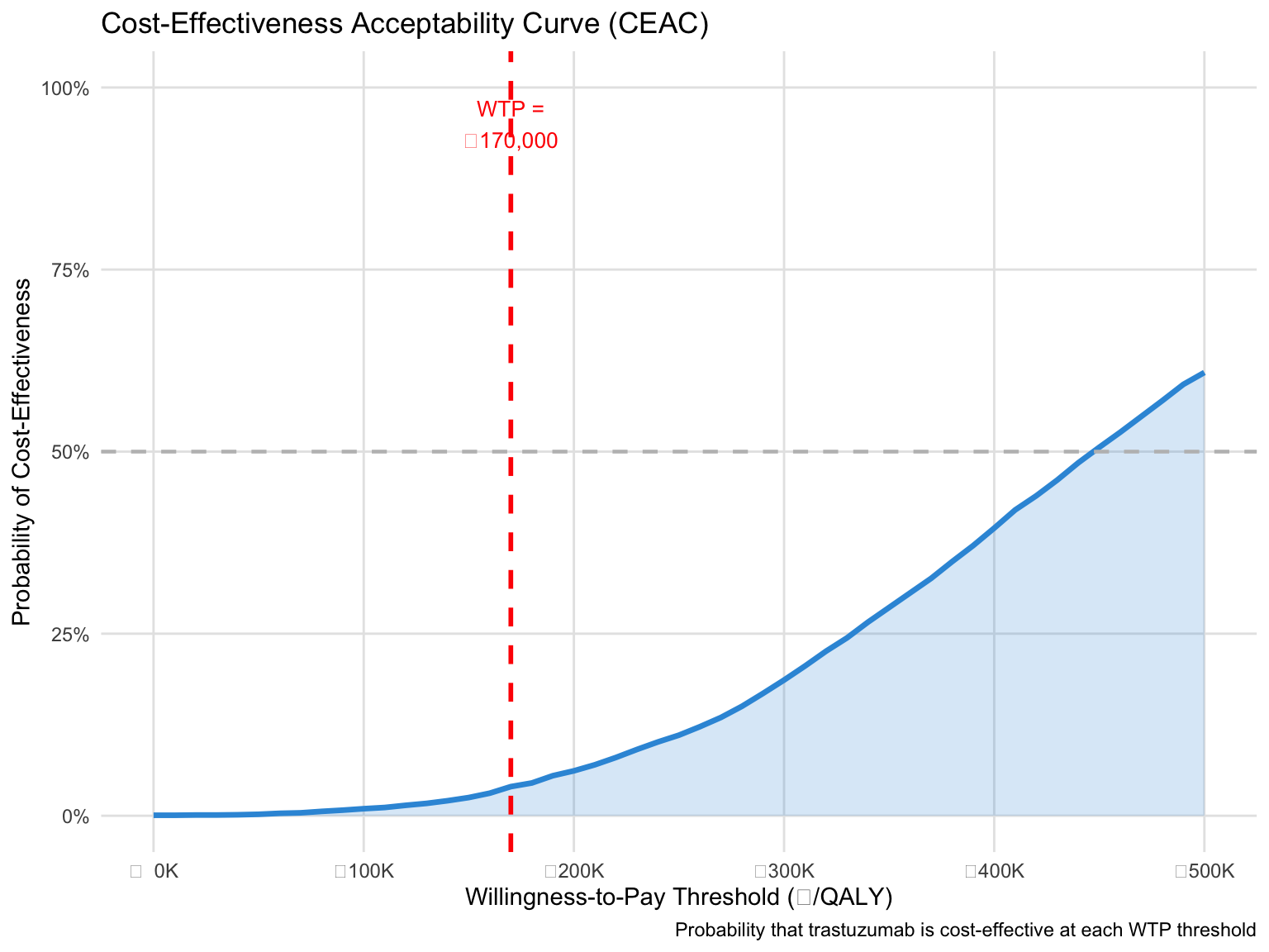
## Cost-Effectiveness Acceptability Curve (CEAC)
The CEAC shows the probability that trastuzumab is cost-effective across a range of WTP thresholds.
```{r}
#| fig-width: 8
#| fig-height: 6
# Calculate CE probability at range of WTP thresholds
wtp_range <- seq(0, 500000, by = 10000)
ce_prob <- sapply(wtp_range, function(wtp) {
  mean(psa_results$inc_cost <= (wtp * psa_results$inc_qaly))
})

ceac_df <- tibble(
  wtp = wtp_range,
  prob_ce = ce_prob
)

# CEAC plot
p_ceac <- ggplot(ceac_df, aes(x = wtp, y = prob_ce)) +
  geom_line(linewidth = 1.2, colour = "#3498db") +
  geom_ribbon(aes(ymin = 0, ymax = prob_ce), alpha = 0.2, fill = "#3498db") +
  geom_vline(xintercept = 170000, linetype = "dashed", colour = "red", linewidth = 1) +
  geom_hline(yintercept = 0.5, linetype = "dashed", colour = "grey", linewidth = 0.8) +
  annotate("text", x = 170000, y = 0.95,
           label = "WTP =\n₹170,000", hjust = 0.5, size = 3.5, colour = "red") +
  labs(
    title = "Cost-Effectiveness Acceptability Curve (CEAC)",
    x = "Willingness-to-Pay Threshold (₹/QALY)",
    y = "Probability of Cost-Effectiveness",
    caption = "Probability that trastuzumab is cost-effective at each WTP threshold"
  ) +
  scale_x_continuous(labels = function(x) paste0("₹", format(round(x/1e3), big.mark = ","), "K")) +
  scale_y_continuous(limits = c(0, 1), labels = scales::percent) +
  theme(
    axis.text.x = element_text(size = 9)
  )

print(p_ceac)
```
## Key Findings
1. **NMB over ICER for PSA**: The mean incremental NMB gives an unambiguous answer — positive means adopt. Unlike the ICER, NMB can be safely averaged and compared across iterations without distortion from extreme values.
2. **Cost-effectiveness at ₹170,000/QALY**: The P(cost-effective) directly answers the decision-maker's question: "Given our uncertainty, how confident can we be that this is a good investment?"
3. **Uncertainty drivers**: Survival uncertainty (hazard ratio distributions) drives most of the ICER/NMB spread. Cost uncertainty is substantial but has a smaller effect — this tells us where to invest in better data.
4. **Decision robustness**: If P(cost-effective) > 80%, the evidence is strong. If 50–80%, there's meaningful decision uncertainty. Below 50%, the intervention is probably not cost-effective at that WTP.
## Comparison with Session 6 PSA
Both Session 6 (Markov model) and this session (PSM) used identical PSA methodology:
- Define parameter distributions
- Sample from those distributions
- Run model with sampled parameters
- Collect and summarize results
**The key lesson: PSA methodology is independent of model structure.** Whether you build a Markov model, a state-transition model, a partitioned survival model, or a discrete event simulation, the PSA approach remains the same. What changes is the model function that gets called with sampled parameters.
## References
- Briggs, A., Claxton, K., & Sculpher, M. (2006). Decision Modelling for Health Economic Evaluation. Oxford University Press.
- Husereau, D., Drummond, M., Petrou, S., et al. (2022). Consolidated Health Economic Evaluation Reporting Standards (CHEERS) 2022 Explanation and Elaboration. *Value in Health*, 25(1), 10-31.
- Fenwick, E., O'Brien, B. J., & Briggs, A. (2001). Cost-effectiveness acceptability curves - facts, fallacies and frequently asked questions. *Health Economics*, 10(7), 605-606.
- National Institute for Health and Care Excellence (NICE). (2022). Guide to the methods of technology appraisal 2022. https://www.nice.org.uk/guidance/gid-tag534/documents